Download
1 / 35
350 likes | 439 Views
Explore the science objectives and measurement requirements for GEO-CAPE, focusing on ozone sensitivity, air quality forecasts, and pollution monitoring. Learn about instrument designs and strategies to meet GEO-CAPE objectives. 8

E N D
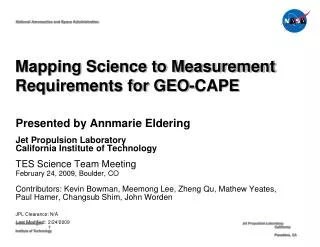
National Aeronautics and Space Administration Mapping Science to Measurement Requirements for GEO-CAPE Presented by Annmarie Eldering Jet Propulsion Laboratory California Institute of Technology TES Science Team Meeting February 24, 2009, Boulder, CO Contributors: Kevin Bowman, Meemong Lee, Zheng Qu, Mathew Yeates, Paul Hamer, Changsub Shim, John Worden JPL Clearance: N/A Last Modified: 2/24/2009 www.nasa.govJet Propulsion Laboratory 1 California Institute of Technology Pasadena, CA
Introduction to GEO-CAPE From the decadal survey, GEO-CAPE science objectives -
GEO-CAPE Science Objectives Geostationary orbit enables continuous continental & regional observations
Practically designing a mission • Take broad science objectives and ….. • Develop specific measurement requirements (species, precision, accuracy, vertical resolution, temporal resolution) • Develop instrument designs that can meet the measurement requirements • Identify strategy for using instrument to meet science goals (observation scenario and mission design) OSSE: The ozone case
CMAQ Prior to use of TES CMAQ Using TES Boundary Conditions Why GEO-CAPE needs advances: • GEO-CAPE science questions with societal impacts push us towards a new way of measuring ozone • Improve air quality forecast skill • Quantify impacts of pollution transport on regional to continental scales • Monitor pollution emissions • Current measurements fall short for these science goals • Limited sensitivity to the lower layers of the atmosphere • Observations at best twice per day OSSE: The ozone case
Key Questions for GEO-CAPE • Vertical resolution and boundary layer sensitivity, especially with regard to ozone – do we need it, can we do it? • Is rule of thumb of hourly resolution driven by science? • Toolsets: • Simulated retrievals and sensitivity tests • OSSEs that marry retrievals and assimilation to see impact of measurements • adjoints to quantify relationships of measurement variables and science variables OSSE: The ozone case
Suggestions in the literature • Simulations based on existing instrument configurations (TES+OMI) show that combination of UV/vis and IR should have better sensitivity to the boundary layer (Worden et al, 2007; Landgraf & Hasenkamp, 2007). • We have extended this to test in wide range of atmospheric conditions, range of mission designs, and in end-use science applications OSSE: The ozone case
Update model Model prediction Observation operator Estimated fields or parameters Estimate model fields or parameters - Geophysical parameter estimation Sampled geophysical fields Propagation to instrument Observations Exploiting OSSEs in the Mission Design Process Assimilation System - Compare science metrics Reference model fields Instrument model Spatio-temporal sampling OSSE: The ozone case
Our experiments • First phase focused on getting the right instrument sensitivity • In second phase, will study mission design in more detail • How we compare instrument & mission ideas: Averaging kernels - are they sensitive in the region of interest? Bias statistics - does the bias meet the requirements? Maps of characteristics - will the spatial characteristics meet science goals? Assimilate into model - assess ability to capture features of interest Air quality forecast - test ideas against forecast skill OSSE: The ozone case
OMI AIRS TES Instrument designs evaluated UV instruments IR instruments • Using instrument designs in the realm of EOS capabilities. • First plots focus on 6 combinations • IR: 970-1080 cm-1 • UV/vis: 312-344 nm better OSSE: The ozone case
SimulationSampling • Use GEOS-CHEM and regional model fields and geostationary viewing • Assimilate into GEOS-CHEM OSSE: The ozone case
Metrics in our Analysis • Pdf of truth – retrieved • Used to derive bias (mean value of pdf) • - And rms (rms of distribution) OSSE: The ozone case
Can we design an instrument to measure O3 to 5ppb at 825 hPa?? IR only UV only OSSE: The ozone case
Combinations Combo - high noise, low res Combo - low noise, high res OSSE: The ozone case
Looking over the range of cases bias • Lower spectral resolution IR instrument (used alone or in combination with UV/vis) have large bias and rms • Combined high-spectral resolution IR and uv/vis have low bias and rms Rms OSSE: The ozone case
Next Steps • Complete analysis of cross-over region (3.2 and 3.6 micron) for ozone • Extends to other molecules – how important is SO2 to the science of GEO-CAPE, can a joint retrieval improve sensitivity?? • Concept extends beyond GEO-CAPE to many molecules • CO – explored by MOPITT • CO2 and CH4 – we may see some interesting information from GO-SAT OSSE: The ozone case
Assimilation of Simulated Data • Current OSSE includes assimilation into GEOS-CHEM (2 by 2.5 degrees). • We can look at impact of simulated measurements on ozone at various levels of the atmosphere – will the measurements help us answer our science questions? • What is the impact of only a GEO measurement versus GEO plus a LEO?? • Assimilation opportunities – multiple species (ozone and precursors) and regional models OSSE: The ozone case
Sensitivity between states or parameters The sensitivity between states can be calculated this way or that way
Sensitivity Analysis: August 1st, 2006, sensitivity of NY ozone at 2:30 pm to its precursors region of maximum sensitivity of boundary layer ozone in New York to free tropospheric NOx target region The sensitivity of ozone in NY to free tropospheric NOx on 7/29/06 over Chicago is roughly half of the sensitivity to local NOx on 08/01/06
How sensitive is ozone to local NOx? Strong diurnal variation Boundary layer ozone is sensitive to local NOx up to 3 days before Highest sensitivity to morning NOx
Does knowing free tropospheric ozone improve boundary layer ozone prediction? The maximum sensitivity of ozone in NY to free tropospheric ozone is roughly .2 two days before.
Does knowing ozone today improveozone predictability for the following day? The sensitivity of ozone to ozone on 07/31/08 is about half of ozone on 08/01/08
Conclusions • It is critical to tie the science questions to measurement requirements and then instrument requirements for GEO-CAPE • We have toolset for quickly making a relative comparison of nadir viewing instruments designs for atmospheric composition with simulated retrievals, assimilation, and adjoints • Analysis suggests that boundary level ozone can be measured with UV/vis paired with high spectral resolution (0.06) IR with good noise characteristics • Mission design (footprint size, frequency of measurements) to be evaluated in geostationary framework • More analysis by atmospheric sciences community important to develop consensus and move GEO-CAPE forward OSSE: The ozone case
BACKUP OSSE: The ozone case
Outline: • Motivation: Measuring tropospheric pollution and air quality from space for GEO-CAPE • Approach: Evaluation of possible approaches for ozone – focused on 825 hPa • Conclusion • There are instrument designs that can measure boundary layer ozone • Use of uv/vis and high spectral resolution IR wavelengths together are needed to have low bias and low rmsin 825 hPa ozone • GEOS-CHEM adjoint being used to quantify spatial and temporal relationships OSSE: The ozone case
Comparing statistics: varying width of IR window UV + IR IR only Bias: 1.46 rms: 14.6 Bias: 0.87 rms: 6.03 Bias: -4.42 rms: 16.9 UV only Narrow window 1043-1075 Bias: -2.44 rms: 15.4 Bias: -0.02 rms: 6.51 wider window 970-1080 OSSE: The ozone case
Preparing to include 3.6 microns • Need to perform radiative transfer calculations with both solar terms and thermal emission OSSE: The ozone case
Verifying RT calculations in LIDORT Wavenumber (2778 cm-1 = 3.6 microns) OSSE: The ozone case
Next Steps • Complete characterizations of 3.6 micron window • combine with UV/vis and IR • break down UV/vis into more specific bands (as Kelly Chance has outlined) OSSE: The ozone case
Sampling the field + retrievals Orbiter-2D • Can select orbit parameters and footprints, profiles then selected from field. • Generate radiance, apply instrument function, and use linearized optimal estimation to generate simulated retrievals and error characterization (as well as averaging kernels). OSSE: The ozone case
For one simulation, histogram of error For one simulation, distribution of error Comparing requirements to simulated performance Mean bias @ 825hPa for all simulated instruments Focus on the ozone requirements from the NRC white paper - JANZ All figures for 825 hPa OSSE: The ozone case Yellow box marks requirement
CMAQ Prior to use of TES CMAQ Using TES Boundary Conditions Where do we go from here? • Important science questions with societal impacts push us towards a new way of measuring ozone (GEO-CAPE) • Improve air quality forecast skill • Quantify impacts of pollution transport on regional to continental scales • Monitor pollution emissions • Current measurements fall short for these science goals • Limited sensitivity to the lower layers of the atmosphere • Observations at best twice per day OSSE: The ozone case
Suggestions in the literature • Simulations based on existing instrument configurations (TES+OMI) show that combination of UV/vis and IR should have better sensitivity to the boundary layer. • We have extended this to test in wide range of atmospheric conditions, range of mission designs, and in end-use science applications OSSE: The ozone case
Science question used to define measurement requirements Instrument designed to meet measurement requirements (sensitivity) Mission designed to meet measurement requirements (frequency of samples) Thoroughly test in simulated science analysis Using OSSEs to more fully evaluate possible approaches (getting to the right design for the INSTRUMENT and the MISSION): OSSE: The ozone case
Measuring ozone from Space • We have a long history of space based measurements • Many nadir viewing approaches, key for tropospheric measurements • Total column ozone from SBUV, TOMS, and OMI based on uv/vis • GOME, SCIAMACHY, GOME-2 • Infrared sounder measurements • AIRS total column • TES - profiles with ability to differentiate the upper and lower troposphere • IASI - total columns and some thick layer vertical information OSSE: The ozone case