Download

1 / 22
220 likes | 322 Views
Explore key science drivers in helioseismology for understanding solar dynamics, including vorticity, subsurface structures, magnetic oscillations, and space weather forecasts. Dive into deep meridional flow inversion and the influence of solar cycles on patterns such as poleward and equatorward flows. Investigate the challenges and potentials of cross-spectral helioseismology for enhanced frequency accuracy and atmospheric insights. Examine magneto-seismology for magnetic oscillations and validation using far-side helioseismic maps. Incorporate far-side observations into space weather forecasting models, such as the ADAPT system, to improve solar wind speed predictions.

E N D
Science Requirements for Helioseismology Frank Hill NSO SPRING Workshop Nov. 26, 2013
Science drivers • Understand dynamics below active regions – vorticity, divergence • Continue observations of large-scale zonal and meridional flows underlying the dynamo and solar activity • Continue measurement of frequency variations during the cycle – is there a near-surface dynamo? • Correctly infer the structure below active regions • Improve the precision and accuracy of mode property measurements to improve inferences of solar interior • Further understand mode excitation and damping • Probe solar atmosphere structure and dynamics – are there acoustic cavities? • Investigate magnetic field oscillations – magnetoseismology • Investigate relationship between active region magnetic field direction and subsurface flows • Develop space-weather forecasts from helioseismology
Deep Meridional Flow Inversion Inversion of meridional flow measurements using 3 years of GONG data (2007-2009). Top: Flow map as a function of latitude and depth . Color convention: red – poleward flow, blue – Equatorward. Bottom: Average (10 < lat < 30 deg) meridional flow speed as a function of depth. Deep return meridional flow with amplitude about 5 m/s is clearly seen. Multi-cell structure in depth is visible, but requires many more measurements to get robust depth profile. This result is obtained after systematic East-West travel time corrections have been subtracted.
Cycle 24 (2009-2020?) Poleward branch Equatorwardbranch Where is Cycle 25??? 2023?-2034? Cycle 23 (1995-2009) Equatorward Branch Change in differential rotation has hidden weak Cycle 25 poleward branch
Upper panel: GONG oscillation frequency shifts over solar cycle 23 averaged over 0 ≤ℓ≤ 120 for two frequency bands: low (green) and high (red). Lower panel: high-pass filtered data showing ~2 yr cycles which may be the signature of a near-surface dynamo (Simoniello et al. 2012)
“Coffee Cup” Active region subsurface wave speed structure Red – high speed (hot) Blue – low speed (cold)
P modes and inclined magnetic fields Acoustic modes are transformed into various MHD modes when they encounter the level at which the the sound speed and the Alfven speed are equal. The ray paths and energy partition depends on the strength of the magnetic field, the inclination of the magnetic field, the acoustic mode attack angle, and the frequency. This strongly affects the observed relative phases and thus travel times between observed waves that are not actually purely acoustic. Cally 2007
Numerical travel time perturbations at 3 (left), 4 (middle) and 5 (right) mHzas functions of field inclination θ and wave orientation attack angle φ
Cross- spectral helioseismology • Cross-spectral analysis should provide more accurate frequencies • E.g. simultaneous four-spectra fitting (PI, Pv, CIV, φIV) • Phase differences provide information on excitation & damping • Phase differences provide information on atmospheric structure and possible acoustic cavities Barban, Hill & Kras, 2004
Magnetic oscillations at disk center for the period 2008 August 1-28: (Top) Cross-sectional cuts of three-dimensional ring diagram power spectra at 3.333 mHz. (Bottom) The asymmetry parameter as a function of frequency obtained from spherical harmonic decomposition for ℓ = 275. But is it the Sun or instrumental cross-talk?
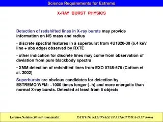
Validation of GONG Far-Side Helioseismic Maps by comparison with STEREO observations Liewer, P. C., et al., 2012, “Comparison of Far-Side STEREO Observations of Solar Activity and Active Region Predictions from GONG”, SoPh “…. we found that for 139 of 157 (89%) comparisons, STEREO EUVI showed a bright region, indicating activity, at the location of the GONG predicted far-side active regions. Only 11% of the predictions showed no significant brightening in either 195 Å or 304 Å images.” “In this study, we identified 15 large active regions that appeared on the east limb (as seen from Earth) between 1 February and 20 July 2011. GONG successfully predicted eight of these 15 regions (55%) with a confidence level higher than 70%. “
Incorporating Far-Side Observations into ADAPT for Space Weather Forecasting Diagram of the general data flow and processing of ADAPT: Data Assimilator F10.7 forecasting using ADAP maps with and without far-side information. Henney, C. et al (26th NSO Workshop presentation, May 2012) ADAPT Input Data Modeling / Forecasting Applications Solar Magnetogram Data Intelligent Front End Initial Conditions Coronal & Solar Wind Models Improved Solar Synoptic Maps Forecast Step: use the WH model tocalculate forecast Import & Select Data for Data Assimilator Polarity + Error Estimation Improvements is Solar Wind forecasting using the far-side data Solar wind speed observations from STEREO B (black solid lines) vs. 4-day WSA predictions (blue dots) using daily ADAPT maps without the far-side active region included (a). The lower time series (b) is the same as (a) except now using ADAPT maps with the far-side active region from the seismic maps included. The red vertical bars indicate the range over which WSA solar wind speed predictions vary over a grid cell. (courtesy of C.N. Arge) Analysis Step: combine observations with forecast Global Magnetic Field WSA-ENLIL Solar Wind Magnetic Field Variance Far-side map Assimilation Results
Pre-emergence active region detection Deep focusing travel-time maps of AR 10488. The focus depth covers 40-70 Mm. Each map is created using 8-hours of MDI data centered at the emerging AR location. The color scale in the travel-time maps covers the perturbation range 0 (blue) to -15 (red) sec. Last three panels: magnetic field for time period of the first panel in the middle row; for time period when AR emerged to the surface; and intensity map for three days. Only a few active regions have been detected using this technique.
Science requirements • Continue what we do now so solar cycle-related flows are adequately captured and space weather forecasts are enabled: • Full-disk Doppler velocity • Cadence of no longer than 60 seconds • 90% duty cycle • 25 year lifetime • Sufficient overlap with current data for cross-calibration • Go beyond what we do now: • Multiple heights for mode conversion, cross-spectral fitting and atmospheric seismology • Vector magnetic field for mode conversion and magnetoseismology • Increase spatial resolution to observe higher latitudes • Increase numerical simulation efforts to understand and guide observations
Multi-wavelength oscillation power, phase, coherence maps from SDO Data provides info on wave properties as function of height, needed to provide reliable active region structure inversions. Note that the high-freq. phase in quiet Sun does not reflect assumed order of formation heights, as expected for upward-traveling waves; HMI IL shows a larger phase shift relative to HMI V than does AIA 1700 Å. Likely cause is MHD mode conversion.
Technical requirements • Observations in multiple spectral lines e.g.: • Ni I 6768 (GONG, MDI) • Fe I 6301/2 (magnetic field) • CA 8542 (Chromosphere) • Fe I 6173 (HMI) • Images of 4k 4k pixels (1” resolution) • Velocity sensitivity: 1 m/s /pixel /image (?) • Magnetic field sensitivity: 5 G /pixel /image (?) • Entrance aperture of at least 0.5 m • Adaptive optics or other image enhancement technology • High-speed image post-processing • Instruments located at least six sites • Highly accurate N-S alignment of instruments • High-speed real-time data return via the internet