Download
1 / 21
210 likes | 305 Views
Explore the cutting-edge Wetlands Analysis and Assessment Mapper (WAAM) methods used in the Randolph County study to evaluate hyperspectral image data, enhanced wetland identification methods, and compare traditional mapping techniques. The research partnership between EarthData, MSU, and NC DOT leveraged LIDAR technology for precise DEM production, hydrologic analysis, and vegetation assessment.

E N D
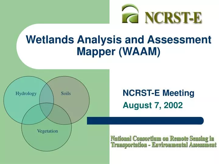
Wetlands Analysis and Assessment Mapper (WAAM) NCRST-E Meeting August 7, 2002 Hydrology Soils Vegetation
NEPA StreamliningRandolph County, North Carolina For EarthData’s “NEPA Streamlining TAP” in Randolph County, NC, MSU, EarthData, ITRES, and NC DOT developed a research partnership wherein MSU was asked to develop research to accomplish the following tasks: • Evaluate new hyperspectral image, elevation, and hydrologic data; • Develop enhancements for wetland identification methods; and • Evaluate the differences between traditional wetland mapping techniques for assessment.
Hyperspectral Image and Wetland Data CollectionRandolph County, North Carolina Hyperspectral image data were collected andclassified to obtain classes that closely resembled those used in NWI surveys.
LIDAR Data and Derived DEM and Hydrologic Information Products A high-resolution digital elevation model (DEM) was produced for the analysis development area using data collected by EarthData’s airborne LIDAR system. The LIDAR data were evaluated for preliminary design as well as cut and fill analyses for roadway construction. Typical DEM products such as USGS 1:24,000 scale DEMs are generally not of sufficient quality for roadway design and construction analysis. However, the quality of information products that can be developed with LIDAR show much promise for topographic, morphologic, and hydrologic analysis as well as for preliminary roadway design.
Clarifying Stratified Data The methods developed for vegetation analysis were designed to consider the pixels within the ¼ acre neighboring area. This was accomplished by specifying a circular focal neighborhood with a radius of 18 one-meter pixels around each pixel. The resultant area is approximately 1017 square meters or about ¼ of an acre.
WAAM Algorithm Development Quantitatively assessing the likelihood of wetlands occurrence required ranking and combining information wetlands criteria layers for vegetation, soils, and hydrology. For this analysis, the data products were grouped into vegetation and non-vegetation information items. Soils and hydrology information products combined to contribute 30 possible points and the vegetation information products combined to contribute 30 possible points.
Neighborhood Vegetation Analysis Techniques The neighborhood vegetation analysis techniques were developed to assess the most significant vegetative component for the neighboring area around each classified image pixel, the weighted sum of components, and the combined dominants present in the neighboring area. • Most Significant Component (MSC): Focal Majority • Weighted Sum of Components (WSC): Focal Sum • Combined Dominants (CD): Combination of Focal Counts
Vegetation Information The VI product is generated from the high-spatial resolution hyperspectral classified image data analysis products. The MSC, WSC, and CD analysis products are ranked from 0 to 10 and combined to produce the VI information product.
Hydrologic Information Products The DEM created for the analysis development unit was used for hydrologic analysis. To conduct hydrologic analysis from a DEM, data derivatives must be generated. These include a filled surface so that water can properly flow on all areas of the surface. From the filled surface several other data sets are generated including flow direction and flow accumulation.
Hydrologic Depressions (Sinks) Hydrologic depressions occur in areas where water can flow in, but becomes “trapped” because there are no lower elevation “cells” in the local area to which the water may flow. The raw DEM was subtracted from a “filled” DEM to create a “sinks” surface. Sinks approximate the location and size of hydrologic depressions where surface water is likely to become ponded and stand on the land surface.
Riparian Buffer Zone The stream network was buffered to include an 18-meter distance (radius for a 1/4 acre focal area) from the theoretical drainage centerline that represents the transitional or riparian zone. Within the study area, wetlands along streams are typically completely hidden by the canopy of trees that thrive in this transitional environment.
NRCS County Soils Data The U.S. Department of Agriculture, Natural Resource Conservation Service (NRCS) maps county soils information and the data may be available as a digital product (SSURGO). In this analysis, digital county soils data were used to form a hydric soils layer.
Non-Vegetation Information Layers The combination of non-vegetation information products illustrates the spatial overlay of stream and riparian zones, areas likely to pond overland flow, and soils typical of the wetland environment.
Non-Vegetation Items (NVI) The NVI product is generated from the topographic sinks, transitional zones, and hydric soils data layers. Each layers is ranked either as 10 for presence of topographic sinks, transitional zones, and hydric soils or as 0 for absence.
TPS and PPS The TPS and the PPS created by summing the VI and NVI are useful for comparison with existing data, for early screening of potential wetland areas, for planning field work, and for generating an alignment that travels the “least cost path” across either the TPS or PPS when used as resistance surfaces.
TPS20 To estimate the areas that have a high likelihood of being wetlands it is necessary to define a threshold above which will be considered “high likelihood.” The value “20” represents one-third of the total possible sum, and it is reasonable to assert that areas that exceed a TPS of 20 have a high likelihood of meeting one out of three wetland criteria.
Comparison and Tabulation of Geospatial Agreement When compared to the results of the conventional NWI and NC DOT wetland mapping methods, over 95% of the areas mapped as NWI wetlands or NC DOT’s Field Wetland Assessment areas were within 4 analysis cells of the areas predicted as having a high likelihood of wetlands (TPS20).
Conclusions • Remotely sensed data can be used to perform analysis of the likelihood of wetlands. • MSU is looking at IP aspects of the algorithm. • High-spatial resolution, hyperspectral digital data can be used to generate detailed land cover and vegetation information. • The process is being duplicated in Eddyville, Iowa as reported by Louis and the field and RS data have all been acquired and are being processes. • The CSX railroad relocation will likely use the wetlands analysis algorithm to identify areas with a high wetlands likelihood.