Download
1 / 50
530 likes | 808 Views
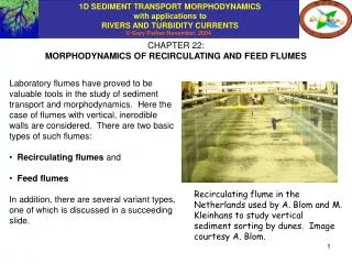
CHAPTER 22: MORPHODYNAMICS OF RECIRCULATING AND FEED FLUMES. Laboratory flumes have proved to be valuable tools in the study of sediment transport and morphodynamics. Here the case of flumes with vertical, inerodible walls are considered. There are two basic types of such flumes:

E N D
CHAPTER 22: MORPHODYNAMICS OF RECIRCULATING AND FEED FLUMES • Laboratory flumes have proved to be valuable tools in the study of sediment transport and morphodynamics. Here the case of flumes with vertical, inerodible walls are considered. There are two basic types of such flumes: • Recirculating flumes and • Feed flumes • In addition, there are several variant types, one of which is discussed in a succeeding slide. Recirculating flume in the Netherlands used by A. Blom and M. Kleinhans to study vertical sediment sorting by dunes. Image courtesy A. Blom.
Neglect entrance and exit regions H S THE MOBILE-BED EQUILIBRIUM STATE The flume considered here is of the simplest type; it has a bed of erodible alluvium, constant width B and vertical, inerodible walls. The bed sediment is covered by water from wall to wall. One useful feature of such a flume is that if it is run long enough, it will eventually approach a mobile-bed equilibrium, as discussed in Chapter 14. When this state is reached, all quantities such as water discharge Q (or qw = Q/B), total volume bed material sediment transport rate Qt (or qt = Qt/B), bed slope S, flow depth H etc. become spatially constant in space (except in entrance and exit regions) and time. (The parameters in question are averaged over bedforms such as dunes and bars if they are present.)
THE EQUILIBRIUM STATE: REVIEW OF MATERIAL FROM CHAPTER 14 The hydraulics of the equilibrium state are those of normal flow. Here the case of a plane bed (no bedforms) is considered as an example. The bed consists of uniform material with size D. The governing equations are (Chapter 5): Water conservation: Momentum conservation: Friction relations: where kc is a composite bed roughness which may include the effect of bedforms (if present). Generic transport relation of the form of Meyer-Peter and Müller for total bed material load: where t and nt are dimensionless constants:
THE EQUILIBRIUM STATE: REVIEW contd. In the case of the Chezy resistance relation, for example, the equations governing the normal state reduce to: In the case of the Manning-Stickler resistance relation, the equations governing the normal state reduce with to: Let D, kc and R be given. In either case above, there are two equations for four parameters at equilibrium; water discharge per unit width qw, volume sediment discharge per unit width qt, bed slope S and flow depth H. If any two of the set (qw, qt, S and H) are specified, the other two can be computed.
THE RECIRCULATING FLUME In a recirculating flume all the water and all the sediment are recirculated through a pump. The total amounts of water and sediment in the system are conserved. In addition to the sediment itself, the operator is free to specify two parameters in operating the flume: the water discharge per unit width qw and the flow depth H. The water discharge (and thus the discharge per unit width qw) is set by the pump setting. (More properly, what are specified are the head-discharge relation of the pump and the setting of the valve on the return line, but in many recirculating systems flow discharge itself can be set with relative ease and accuracy.) The constant flow depth H reached at equilibrium is set by the total amount of water in the system, which is conserved. Increasing the total amount of water in the system increases the depth reached at final mobile-bed equilibrium. Thus in a recirculating flume, equilibrium qw and H are set by the flume operator, and total volume sediment transport rate per unit width qt and bed slope S evolve to equilibrium accordingly.
THE FEED FLUME In a feed flume all the water and all the sediment are fed in at the upstream and allowed to wash out at the downstream end. Water is introduced (usually pumped) into the channel at the desired rate, and sediment is fed into the channel using e.g. a screw-type feeder at the desired rate. In addition to the sediment itself, the operator is thus free to specify two parameters in the operation of the flume: the water discharge per unit width qwand the total volume sediment discharge per unit width qt reached at final equilibrium, which must be equal to the feed rate qtf. Thus in a feed flume, equilibrium qw and qt are set, by the flume operator, and equilibrium flow depth H and bed slope S evolve accordingly.
A HYBRID TYPE: THE SEDIMENT-RECIRCULATING, WATER-FEED FLUME In the sediment-recirculating, water-feed flume the sediment and water are separated at the downstream end. Nearly all the water overflows from a collecting tank. The sediment settles to the bottom of the collecting tank, and is recirculated with a small amount of water as a slurry. The water discharge per unit width qw is thus set by the operator (up to the small fraction of water discharge in the recirculation line). The total amount of sediment in the flume is conserved. In addition, a downstream weir controls the downstream elevation of the bed. The combination of these two conditions constrains the bed slope S at mobile-bed equilibrium. Adding more sediment to the flume increases the equilibrium bed slope. Thus in a sediment-recirculating, water-feed flume, qw and S are set by the flume operator and qt and H evolve toward equilibrium accordingly.
MORPHODYNAMICS OF APPROACH TO EQUILIBRIUM • The final mobile-bed equilibrium state of a flume is usually not precisely known in advance. Flow is thus commenced from some arbitrary initial state and allowed to approach equilibrium. This motivates the following two questions: • How long should one wait in order to reach mobile-bed equilibrium? • What is the path by which mobile-bed equilibrium is reached? • It might be expected that the answer to these questions depends on the type of flume under consideration. Here two types of flumes are considered: a) a pure feed flume and b) a pure recirculating flume. • In performing the analysis, the following simplifying assumptions (which can easily be relaxed) are made: • The flow is always assumed to be subcritical in the sense that Fr < 1. • The channel is assumed to have a sufficiently large aspect ration B/H that • sidewall effects can be neglected. • Bed resistance is approximated in terms of a constant resistance coefficient • Cf, so that the details of bedform mechanics are neglected. • The sediment has uniform size D. • The analysis presented here is based on Parker (2003).
THE LEGEND OF SEDIMENT LUMPS IN RECIRCULATING FLUMES In the world of sediment flumes, there is a persistent legend concerning recirculating flumes that is rarely documented in the literature. That is, these flumes are said to develop sediment “lumps” that recirculate round and round, either without dissipating or with only slow dissipation. The author of this e-book has heard this story from T. Maddock, V. Vanoni and N. Brooks. One of the author’s graduate students encountered these lumps in a recirculating, meandering flume and showed them to the author (Hills, 1987).
THE LEGEND OF SEDIMENT LUMPS IN RECIRCULATING FLUMES In the world of sediment flumes, there is a persistent legend concerning recirculating flumes that is rarely documented in the literature. That is, these flumes are said to develop sediment “lumps” that recirculate round and round, either without dissipating or with only slow dissipation. The author of this e-book has heard this story from T. Maddock, V. Vanoni and N. Brooks. One of the author’s graduate students encountered these lumps in a recirculating, meandering flume and showed them to the author (Hills, 1987).
THE LEGEND OF SEDIMENT LUMPS IN RECIRCULATING FLUMES In the world of sediment flumes, there is a persistent legend concerning recirculating flumes that is rarely documented in the literature. That is, these flumes are said to develop sediment “lumps” that recirculate round and round, either without dissipating or with only slow dissipation. The author of this e-book has heard this story from T. Maddock, V. Vanoni and N. Brooks. One of the author’s graduate students encountered these lumps in a recirculating, meandering flume and showed them to the author (Hills, 1987).
THE LEGEND OF SEDIMENT LUMPS IN RECIRCULATING FLUMES In the world of sediment flumes, there is a persistent legend concerning recirculating flumes that is rarely documented in the literature. That is, these flumes are said to develop sediment “lumps” that recirculate round and round, either without dissipating or with only slow dissipation. The author of this e-book has heard this story from T. Maddock, V. Vanoni and N. Brooks. One of the author’s graduate students encountered these lumps in a recirculating, meandering flume and showed them to the author (Hills, 1987).
THE LEGEND OF SEDIMENT LUMPS IN RECIRCULATING FLUMES In the world of sediment flumes, there is a persistent legend concerning recirculating flumes that is rarely documented in the literature. That is, these flumes are said to develop sediment “lumps” that recirculate round and round, either without dissipating or with only slow dissipation. The author of this e-book has heard this story from T. Maddock, V. Vanoni and N. Brooks. One of the author’s graduate students encountered these lumps in a recirculating, meandering flume and showed them to the author (Hills, 1987).
PARAMETERS x = streamwise coordinate t = time H = H(x, t) = flow depth U = U(x, t) = depth-averaged flow velocity = (x, t) = bed elevation S = - /x = bed slope g = gravitational acceleration qt = volume bed material sediment transport rate per unit width qw = UH = water discharge per unit width b = boundary shear stress at bed L = flume length B = flume width D = sediment size p = porosity of bed deposit of sediment
KEY APPROXIMATIONS AND ASSUMPTIONS • Flume has constant width B. • Sediment is of uniform size D. • H/B << 1: flume is wide and sidewall effects can be neglected. • Flume is sufficiently long so that entrance and exit regions can be neglected. • Flow in the flume is always Froude- subcritical: Fr = U/(gH)1/2 < 1. • qt/qw << 1: volume transport rate of sediment is always much lower than that of water. • Resistance coefficient Cf is approximated • as constant.
GOVERNING EQUATIONS: 1D FLOW Flow mass balance Flow momentum balance Sediment mass balance Closure relation for shear stress: Cf = dimensionless bed friction coefficient The condition qt/qw << 1 allows the use of the quasi-steady approximation introduced in Chapter 13, according to which the time-dependent terms in the equations of flow mass and momentum balance can be neglected.
REDUCTION TO BACKWATER FORM The equations of flow mass and momentum balance reduce to the standard backwater equation introduced in Chapter 5. or thus where
SEDIMENT TRANSPORT RELATION Sediment transport is characterized in terms of the same generic sediment transport relation as used in Chapter 20, except that the parameter s is set equal to unity. Thus where D = grain size (uniform) s = sediment density = water density R = (s/ ) – 1 1.65 Einstein number Shields number
CONSTRAINTS ON A RECIRCULATING FLUME Water discharge qw is set by the pump. The total amount of water in the flume is conserved. With constant width, constant storage in the return line and negligible storage in the entrance and exit regions (L sufficiently large), the constraint is (where C1 is a constant): At final equilibrium, when H = Ho, the constraint reduces to HoL = C1, according to which Ho is set by the total amount of water. The total amount of sediment in the flume is conserved. Neglecting storage in the return line and the head box, the constraint is (where C2 is another constant): Integrate the equation of sediment mass conservation to get So a cyclic boundary condition is obtained: But from above
Three constraints: CONSTRAINTS ON A FEED FLUME Water discharge qw is set by the pump. The upstream sediment discharge is set by the feeder. Where qtf is the sediment feed rate: Let = + H denote water surface elevation. The downstream water surface elevation d is set by the tailgate: The long-term equilibrium approached in a recirculating flume (without lumps) should be dynamically equivalent to that obtained in a sediment-feed flume (e.g. Parker and Wilcock, 1993).
MOBILE-BED EQUILIBRIUM The equation for water conservation reduces to: At mobile-equilibrium the equation of momentum balance reduce to the relation for normal flow introduced in Chapter 5: The sediment transport relation reduces to the form: which applies whether or not mobile-bed equilibrium is reached. Let R, g, D, t, nt, c* and Cf be specified. The equations in the boxes define three equations in five parameters Uo, Ho, qto, qw and So at mobile-bed equilibrium.
MOBILE-BED EQUILIBRIUM contd. Recirculating flume: Water discharge/width qw is set by pump. Total amount of water Vw in system is conserved. Assuming constant storage in return line and neglecting entrance and exit storage, Vw = HLB depth Ho is set. Solve three equations for qto, U0, So. The subscript “o” denotes mobile-bed equilibrium conditions. Feed flume: Water discharge/width qw is set by pump. Sediment discharge/width qto is set by feeder. Solve three equations for uo, Ho, So.
APPROACH TO EQUILIBRIUM: NON-DIMENSIONAL FORMULATION Dimensionless parameters describing the approach to equilibrium (denoted by the tilde or downward cup) are formed using the values Ho, qto, So corresponding to normal equilibrium. Bed elevation is decomposed into into a spatially averaged value and a deviation from this d(x, t), so that by definition The above two parameters are made dimensionless as follows:; From the above relations, = the dimensionless flume number where
APPROACH TO EQUILIBRIUM contd. The dimensionless relations governing the approach to equilibrium are thus as follows; where Fro and denote the Froude and Shields numbers at mobile-bed equilibrium, respectively, The backwater relation is: The relation for sediment conservation decomposes into two parts: The sediment transport relation is : where
APPROACH TO EQUILIBRIUM IN A FEED FLUME In a feed flume, the boundary condition on the sediment transport rate at the upstream end is , or in dimensionless variables, Thus the relations for sediment conservation of the previous slide reduce to The boundary condition on the backwater equation is where d is a constant downstream elevation set by a tailgate. This condition must hold at all flows, including the final mobile-bed equilibrium. Now the datum for elevation is set (arbitrarily but conveniently) to be equal to the bed elevation at the center of the flume (x = 0.5 L) at equilibrium, so that ao = 0 and Between the above two relations and the nondimensionalizations, it is found that
APPROACH TO EQUILIBRIUM IN A FEED FLUME: SUMMARY The equations must be solved with the sediment transport relation and boundary conditions: and a suitable initial condition, e.g. where SI is an initial bed slope and aI is an initial value for flume-averaged bed elevation, , a = aI, d = SIL[0.5 – (x/L)], or in dimensionless terms. Note furthermore that aI ( ) and SI must be chosen so as to yield subcritical flow in the flume at t = 0 ( ).
APPROACH TO EQUILIBRIUM IN A FEED FLUME: FLOW OF THE CALCULATION In the case of a feed flume, the calculation flows directly with no iteration. At any time (e.g. ) the bed elevation profile, e,g, the parameters and , are known. The backwater equation is then solved for using the standard step method of Chapter 5 upstream from the downstream end, where the boundary condition is: Once is known everywhere, is obtained everywhere from the sediment transport relation of the previous slide. The bed elevation one time step later is determined from a discretized version of where the second equation above is solved subject to the boundary condition
APPROACH TO EQUILIBRIUM IN A RECIRCULATING FLUME As shown at the bottom of Slide 19, the sediment transport in a recirculating flume must satisfy a cyclic boundary condition. In dimensionless terms, this becomes As a result, the relations for sediment conservation of Slide 24 reduce to The total amount of water in the flume is conserved. Evaluating the constant in the equation at the top right of Slide 19 from the final equilibrium, then, In dimensionless form, this constraint becomes
APPROACH TO EQUILIBRIUM IN A RECIRCULATING FLUME: SUMMARY The equation for can be dropped because flume-averaged bed elevation cannot change in a recirculating flume. The remaining backwater and sediment conservation relations must be solved with the sediment transport relation and constraints: The initial condition is where the initial slope SI must be chosen so as to yield subcritical flow everywhere.
APPROACH TO EQUILIBRIUM IN A RECIRCULATING FLUME: FLOW OF THE CALCULATION The method of solution is similar to that for the feed flume with one crucial difference: iteration is required to solve the backwater equation over a known bed subject to the integral condition That is, for any guess it is possible to solve the backwater equation and test to see if the integral condition is satisfied. The value of necessary to satisfy the backwater equation can be found by trial and error, or as shown below, by a more systematic set of methods.
RESPONSE OF A RECIRCULATING FLUME TO AN INITIAL BED SLOPE THAT IS BELOW THE EQUILIBRIUM VALUE The low initial bed slope causes the depth to be too high upstream. Total water mass in the flume can be conserved only by constructing an M2 water surface profile. The result is a shear stress, and thus sediment transport rate at the downstream end that is higher than the upstream end. This sediment is immediately recirculated upstream, where it cannot be carried, resulting in bed aggration there.
RECIRCULATING FLUME: ITERATIVE SOLUTION OF BACKWATER EQUATION The shooting method is combined with the Newton-Raphson method to devise a scheme to solve the backwater equation iteratively. Now for each guess it is possible to solve the backwater equation for , so that in general the solution can be written as Now define the function such that The correct value of is the one for which the integral constraint is satisfied, i.e.
ITERATIVE SOLUTION OF BACKWATER EQUATION contd. Now according to the Newton Raphson method, if is an estimate of the solution for , then a better estimate (where w = 1, 2, 3… is an iteration index) is given as Reducing this relation with the definition of , results in the iteration scheme This iterative scheme requires knowledge of the parameter .
ITERATIVE SOLUTION OF BACKWATER EQUATION contd. Now define the variational parameter Hv as The governing equation and boundary condition of the iterative scheme are Taking the derivative of both equations with respect to results in the variational equation and boundary condition below;
ITERATIVE SOLUTION OF BACKWATER EQUATION contd. For any guess , then, the following two equations and boundary conditions can be used to find and for all values of . The improved guess is then given as The iteration scheme is continued until convergence is obtained.
NUMERICAL IMPLEMENTATION Numerical implementations of the previous formulation for both recirculating and feed flumes are given in RTe-bookRecircFeed.xls. The GUI for the case of recirculation is given in worksheet “Recirc”, and the GUI for the case of feed is given in worksheet “Feed”. The corresponding codes are in Module 1 and Module 2. Both these formulations use a) a predictor-corrector method to compute backwater curves, and b) pure upwinding to compute spatial derivatives of qt in the various Exner equations of sediment conservation. The discretization given below is identical to that used in Chapter 20. The ghost node for sediment feed is not used, however, in the implementation for the recirculating flume.
NUMERICAL IMPLEMENTATION contd. The backwater equation is solved using a predictor-corrector scheme. The solution proceeds upstream from the downstream node M+1, where for a feed flume and for a recirculating flume is obtained from the iteration scheme using the Newton-Raphson and shooting techniques. The discretized backwater forms for dimensionless depth are: In the case of a recirculating flume, the variational parameter Hv must also be computed subject to the boundary condition Hv,M+1 = 1. The corresponding forms are
NUMERICAL IMPLEMENTATION contd. In the case of a feed flume, the discretized forms for sediment conservation are In the case of a recirculating flume, the corresponding form is
CRITERION FOR EQUILIBRIUM It is assumed that equilibrium has been reached when the bed slope is everywhere within a given tolerance of the equilibrium slope So. A normalized bed slope SN that everywhere equals unity at equilibrium is defined as For the purpose of testing for convergence, the normalized bed slope SN,i at the ith node is defined as At equilibrium, then, SN,i should everywhere be equal to unity. The error i between the bed slope and the equilibrium bed slope at the ith node is Convergence is realized when where t is a tolerance. In RTe-bookRecircFeed.xls t has been set equal to 0.01 (parameter “epslope” in a Const statement).
PHASE PLANE INTERPRETATION One way to interpret the results of the analysis is in terms of a phase plane. Let Sup denote the bed slope at the upstream end of the flume, and Sdown denote it at the downstream end, where Further define the normalized slope SN as equal to S/So, so that The initial normalized slope is denoted as SNI. At mobile-bed equilibrium slope S is everywhere equal to the equilibrium value So, so that SN = 1 everywhere. That is, one indicator of mobile-bed equilibrium is the equality In a phase plane interpretation, SN,up is plotted against SN, down at every time step, and the approach toward (1, 1) is visualized. This equilibrium point (1, 1) is called the fixed point of the phase problem.
PHASE PLANE INTERPRETATION contd. The initial condition for the bed profile is S = SI (SN = SNI) everywhere, where SI is not necessarily equal to the mobile-bed equilibrium value So (SNI is not necessarily equal to 1) . For example, in the case SI = 0.5 So, (SN,up, SNdown) begin with the values (0.5, 0.5) and gradually approach (1, 1). An approach in the form of a spiral is usually indicative of damped sediment waves, or lumps.
INPUT PARAMETERS USED IN THE CODES Input for recirculating flume SI = initial bed slope So = equilibrium bed slope Input for feed flume
SAMPLE CALCULATION WITH RTe-bookRecircFeed.xls: RECIRCULATING FLUME final equilibrium This calculation requires a dimensionless time of 11.94 in order to reach mobile-bed equilibrium. The spiralling is indicative of a damped sediment wave or lump. This is shown in more detail in the next slide. initial
SAMPLE CALCULATION WITH RTe-bookRecircFeed.xls: FEED FLUME final equilibrium The input parameters are comparable to that of the previous case of recirculation. Mobile-bed equilibrium is reached in a dimensionless time of only 4.33. The phase diagram shows no spiralling. initial
APPLICATION EXAMPLE The dimensionless numbers of the previous two calculations, i.e. Fro = 0.4, nt = 1.5, Fl = 10, = 3, SNI = 0.5 and = 0 (feed case only) are now converted to dimensioned numbers for a sample case, for which D = 1 mm, R = 1.65 ks = 2.5 D Ho = 0.2 m (equilibrium depth) The sediment is assumed to move exclusively as bedload. The assumed bedload relation, given below, is from Chapter 6. The assumed resistance relation, given below, is from Chapter 5. From Ho, ks and the above resistance relation, Cf = 0.00354 From Ho and Fro = 0.4, qw = 0.560 m2/s From = 3, o* = 0.148 From o*, D, R and the load relation, qto = 1.57 x 10⁻⁵ m2/s From o* = HoSo/(RD), Ho, R and D, So = 0.00122 From Fl = Ho/(SoL), Ho and So, L = 16.3 m
APPLICATION EXAMPLE contd. In the example, then, the equilibrium parameters are qw = 0.560 m2/s Ho = 0.2 m So = 0.00122 qto = 1.57 x 10⁻⁵ m2/s (= 1250 grams/minute for a flume width B = 0.5 m and the flume length is L = 16.3 m The time to equilibrium tequil is related to the corresponding dimensionless parameter as Assuming the value for bed porosity p of 0.4, the time to equilibrium for the rercirculating case of Slide 43 and the feed case of Slide 45 are then Recirculating flume: tequil = 41.3 hours Feed flume: tequil = 15.0 hours
SOME CONCLUSIONS The following tentative conclusions can be reached concerning sediment lumps in flumes. • Cyclic lumps do occur in recirculating flumes. • These lumps do eventually dissipate. • Similar cyclic lumps are not manifested in sediment-feed flumes. • Feed flumes reach mobile-bed equilibrium faster than recirculating flumes. • Both flume types eventually reach the same mobile-bed equilibrium.
1D SEDIMENT TRANSPORT MORPHODYNAMICS with applications to RIVERS AND TURBIDITY CURRENTS REFERENCES FOR CHAPTER 22 Hills, R., 1987, Sediment sorting in meandering rivers, M.S. thesis, University of Minnesota, 73 p. + figures. Parker, G., 2003, Persistence of sediment lumps in approach to equilibrium in sediment-recirculating flumes, Proceedings, XXX Congress, International Association of Hydraulic Research, Thessaloniki, Greece, August 24-29, downloadable at http://cee.uiuc.edu/people/parkerg/conference_reprints.htm . Parker, G. and Wilcock, P., 1993, Sediment feed and recirculating flumes: a fundamental difference, Journal of Hydraulic Engineering, 119(11), 1192‑1204.