Background

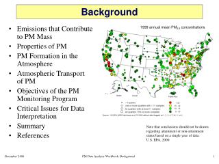
1. Background 1999 annual mean PM2.5 concentrations • Emissions that Contribute to PM Mass • Properties of PM • PM Formation in the Atmosphere • Atmospheric Transport of PM • Objectives of the PM Monitoring Program • Critical Issues for Data Interpretation • Summary • References Note that conclusions should not be drawn regarding attainment or non-attainment status based on a single year of data. U.S. EPA, 2000 PM Data Analysis Workbook: Background

2. Primary PM (directly emitted): Suspended dust Sea salt Organic carbon Elemental carbon Metals from combustion Small amounts of sulfate and nitrate Secondary PM (gases that form PM in the atmosphere): Sulfur dioxide (SO2): forms sulfates Nitrogen oxides (NOx): forms nitrates Ammonia (NH3): forms ammonium compounds Volatile organic compounds (VOC): forms organic carbon compounds Emissions that Contribute to PM Mass PM is composed of a mixture of primary and secondary compounds. PM Data Analysis Workbook: Background

3. NaCl– salt is found in PM near sea coasts, open playas, and after de-icing materials are applied. Organic Carbon (OC) – consists of hundreds of separate compounds containing mainly carbon, hydrogen and oxygen. Elemental Carbon (EC) – composed of carbon without much hydrocarbon or oxygen. EC is black, often called soot. Liquid Water– soluble nitrates, sulfates, ammonium, sodium, other inorganic ions, and some organic material absorb water vapor from the atmosphere. Geological Material – suspended dust consists mainly of oxides of Al, Si, Ca, Ti, Fe, and other metal oxides. Sulfate– results from conversion of SO2 gas to sulfate-containing particles. Nitrate– results from a reversible gas/particle equilibrium between NH3, HNO3, and particulate ammonium nitrate. Ammonium– ammonium bisulfate, sulfate, and nitrate are most common. Major PM2.5 Components Most PM mass in urban and nonurban areas is composed of a combination of the following chemical components: Chow and Watson, 1997 PM Data Analysis Workbook: Background

4. Common PM2.5 Emission Source Profiles (1 of 2) Emission source profiles from EPA SPECIATE for light duty vehicles (profile 31230) and oil-fired power plant (profile 11510). Note differences in Ni and Br, for example. Data are shown using a log scale. (SPECIATE) PM Data Analysis Workbook: Background

5. Common PM2.5 Emission Source Profiles (2 of 2) Emission source profiles from EPA SPECIATE for a municipal incinerator (profile 17106) and Earth’s crust (profile 43309). Note differences in Zn, Cl, S, and Cu, for example. Data are shown using a log scale. (SPECIATE) PM Data Analysis Workbook: Background

6. 88102 Antimony PM2.5 88103 Arsenic PM2.5 88104 Aluminum PM2.5 88107 Barium PM2.5 88109 Bromine PM2.5 88110 Cadmium PM2.5 88111 Calcium PM2.5 88112 Chromium PM2.5 88113 Cobalt PM2.5 88114 Copper PM2.5 88115 Chlorine PM2.5 88117 Cerium PM2.5 88118 Cesium PM2.5 88121 Europium PM2.5 88124 Gallium PM2.5 88126 Iron PM2.5 88127 Hafnium PM2.5 88128 Lead PM2.5 88131 Indium PM2.5 88132 Manganese PM2.5 88133 Iridium PM2.5 88134 Molybdenum PM2.5 88136 Nickel PM2.5 88140 Magnesium PM2.5 88142 Mercury PM2.5 88143 Gold PM2.5 88146 Lanthanum PM2.5 88147 Niobium PM2.5 88152 Phosphorous PM2.5 88154 Selenium PM2.5 88160 Tin PM2.5 88161 Titanium PM2.5 88162 Samarium PM2.5 88163 Scandium PM2.5 88164 Vanadium PM2.5 88165 Silicon PM2.5 88166 Silver PM2.5 88167 Zinc PM2.5 88168 Strontium PM2.5 88169 Sulfur PM2.5 88170 Tantalum PM2.5 88172 Terbium PM2.5 88176 Rubidium PM2.5 88180 Potassium PM2.5 88183 Yttrium PM2.5 88184 Sodium PM2.5 AIRS Codes for PM2.5 88185 Zirconium PM2.5 88186 Wolfram PM2.5 88301 Ammonium Ion PM2.5 88302 Sodium Ion PM2.5 88303 Potassium Ion PM2.5 88305 Organic Carbon PM2.5 88306 Nitrate PM2.5 88307 Elemental Carbon PM2.5 88308 Carbonate Carbon PM2.5 88403 Sulfate PM2.5 PM Data Analysis Workbook: Background

7. Properties of PM • Physical, Chemical and Optical Properties • Size Range of Particulate Matter (PM) • Mass Distribution of PM vs. Size: PM10, PM2.5 • Fine and Coarse Particles • Fine Particles: PM2.5 • Coarse Particle Fraction: PM10-PM2.5; Relationship of PM2.5 and PM10 • Chemical Composition of PM vs. Size • Internal and External Mixtures • Optical Properties of PM Husar, 1999 PM Data Analysis Workbook: Background

8. Physical, Chemical and Optical Properties • PM is characterized by its physical, chemical, and optical properties. • Physical properties include particle size and shape. Particle size refers to particle diameter or “equivalent” diameter for odd-shaped particles. Particles may be liquid droplets, regular or irregular shaped crystals, or aggregates of odd shape. • Particle chemical composition may vary including dilute water solutions of acids or salts, organic liquids, earth's crust materials (dust), soot (unburned carbon), and toxic metals. • Optical properties determine the visual appearance of dust, smoke, and haze and include light extinction, scattering, and absorption. The optical properties are determined by the physical and chemical properties of the ambient PM. • Each PM source type produces particles with a specific physical, chemical, and optical signature. Hence, PM may be viewed as several pollutants since each PM type has its own properties and sources and may require different controls. PM Data Analysis Workbook: Background

9. Size Range of Particulate Matter • The size of PM particles ranges from about tens of nanometers (nm) (which corresponds to molecular aggregates) to tens of microns (70 m  the size of human hair). • The smallest particles are generally more numerous, and the number distribution of particles generally peaks below 0.1 m. The size range below 0.1 m is also referred to as the ultrafine range. • The largest particles (0.1-10 m) are small in number but contain most of the PM volume (mass). The volume (mass) distribution can have two or three peaks (modes). The bi-modal mass distribution has two peaks. • The peak of the PM surface area distribution is always between the number and the volume peaks. Husar, 1999 PM Data Analysis Workbook: Background

10. Mass Distribution of PM vs. Size: PM10, PM2.5 • The mass distribution tends to be bi-modal with the saddle in the 1-3 m size range. • PM10 refers to the fraction of the PM mass 10 m or less in diameter. • PM2.5,or fine mass, refers to the fraction of the PM mass 2.5 m or less in size. • The difference between PM10 and PM2.5 constitutes the coarse fraction. • The fine and coarse particles have different sources, properties, and effects. Many of the known environmental impacts (health, visibility, acid deposition) are attributed to PM2.5. • There is a natural division of atmospheric particulates into fine and coarse fraction based on particle size. Husar, 1999 Fine Coarse PM Data Analysis Workbook: Background

11. Fine and Coarse Particles (1 of 2) Adapted from Seinfeld and Pandis, 1998 PM Data Analysis Workbook: Background

12. Fine and Coarse Particles (2 of 2) • The principal types of secondary particles are ammonium sulfate and ammonium nitrate formed in the atmosphere from gaseous emissions of SO2 and NOx reacting with NH3. • There is a direct relationship between the particle size and the atmospheric residence time of particles: Lyons and Scott, 1990 PM Data Analysis Workbook: Background

13. Fine Particles: PM2.5 • Fine particles ( 2.5 m) result primarily from combustion of fossil fuels in industrial boilers, automobiles, and residential heating systems. • A significant fraction of the PM2.5 mass over the United States is produced in the atmosphere through gas-particle conversion of precursor gases such as sulfur oxides, nitrogen oxides, organics, and ammonia. The resulting secondary PM products are sulfates, nitrates, organics, and ammonium. • Some PM2.5 is emitted as primary emissions from industrial activities and motor vehicles, including soot (unburned carbon), trace metals, and oily residues. • Fine particles are mostly droplets, except for soot which is in the form of chain aggregates. • Over the industrialized regions of the United States, anthropogenic emissions from fossil fuel combustion contribute most of the PM2.5. Biomass burning, windblown dust, and sea salt also contribute. • Fine particles can remain suspended for long periods (days to weeks) and contribute to ambient PM levels hundreds of km away from where they are formed. PM Data Analysis Workbook: Background

14. Spatial Variability of PM2.5 Site correlation of 1999 24-hr average PM2.5 concentrations against distance between sites. Plot prepared using SAS. Data obtained from AIRS on July 12, 2000. Only sites within 100 km were considered; sites had to have at least 10 data pairs matching; no adjustments for different time zones were made. U.S. EPA, 2000 • This analysis characterizes the spatial variability of 24-hr average PM2.5 by calculating the linear correlation coefficients for each possible pair of sites and plotting these as a function of distance. • The correlation remains very high in most of the data out to 100 km. This relationship supports the notion that PM2.5 is a macro-scale or regional pollutant. PM Data Analysis Workbook: Background

15. Coarse Particles: PM10-PM2.5 • Coarse particles (2.5 to 10 m) are generated by mechanical processes that break down crustal material into dust that can be suspended by the wind, agricultural practices, and vehicular traffic on unpaved roads. • Coarse particles are primary in that they are emitted as windblown dust and sea spray in coastal areas. Anthropogenic coarse particle sources include flyash from coal combustion and road dust from automobiles. • The chemical composition of the coarse particle fraction is similar to that of the earth's crust or the sea, but sometimes coarse particles also carry trace metals and nitrates. • Coarse particles are removed from the atmosphere by gravitational settling, impaction to surfaces, and scavenging by precipitation. Their atmospheric residence time is generally less than a day, and their typical transport distance is below a few hundred km. Some dust storms tend to lift the dust to several km altitude, which increases the transport distance to many thousand km. Albritton and Greenbaum, 1998 PM Data Analysis Workbook: Background

16. Relationship of PM2.5 and PM10 (1 of 2) Different areas may have different relationships between PM2.5 and PM10. In this example, the coarse fraction comprises a larger portion of PM10 in the southwestern United States than in the northeasteern United States . U.S. EPA, 2000 PM Data Analysis Workbook: Background

17. Relationship of PM2.5 and PM10 (2 of 2) • PM2.5 and PM10 may have a different relationship during different seasons. • In these examples from 1988, PM2.5 seasonal patterns are similar to those for PM10 in the northeast while seasonal patterns of PM2.5 and PM10 differ in southern California. • PM2.5 comprises a larger fraction of PM10 in the northeastern United States than in southern California. (Note that the concentrations shown in the monthly plots are averages; thus, the sum of fine and coarse concentrations may not equal PM10 concentrations.) Husar, 1999 PM Data Analysis Workbook: Background

18. Chemical Composition of PM vs. Size • The chemical species that make up the PM occur at different sizes. • For example in Los Angeles, ammonium and sulfate occur in the fine mode, 2.5 m in aerodynamic diameter. Carbonaceous soot, organic compounds, and trace metals tend to be in the fine particle mode. • The sea salt components, sodium and chloride, occur in the coarse fraction, > 2.5 m. Windblown and fugitive dust are also found mainly in the coarse mode. • Nitrates may occur in fine and coarse modes. Husar, 1999 PM Data Analysis Workbook: Background

19. Internal and External Mixtures of Particles • During their multi-day atmospheric residence time, particles from different sources and with different compositions are mixed together by a range of atmospheric processes. The resulting particles can be either external or internal mixtures. • In an external mixture, the particle composition will be non-uniform because the components from different sources remain separate (e.g., a soot particle inside a sulfate droplet, as illustrated by the electron micrograph below). • In an internal mixture, the particle composition is uniform because the individual components are completely mixed. • The main process that produces internal mixtures is processing by water such as in fog and/or cloud scavenging and subsequent evaporation. Electron micrograph of a PM2.5 droplet residue. Evidently, the droplet contained a solid particle, possibly soot. Husar, 1999 PM Data Analysis Workbook: Background

20. Optical Properties of PM • Particles effectively scatter and absorb solar radiation. • The scattering efficiency per PM mass is highest at about 0.5 m. This is why, for example, 10 g of fine particles (0.2 < D < 1 m) scatter over ten times more than 10 g of coarse particles (D > 2.5 m). Husar, 1999 PM Data Analysis Workbook: Background

21. PM Formation in the Atmosphere Sulfate Formation in the Atmosphere Sulfate Formation in Clouds Seasonal SO2-to-Sulfate Transformation Rate Residence Time of Sulfur and Organics Nitrate Formation in the Atmosphere Links to Ozone Formation, Health, and Visibility PM Data Analysis Workbook: Background

22. Sulfate Formation in the Atmosphere • Sulfates constitute about half of the PM2.5 in the eastern United States. Virtually all the ambient sulfate (99%) is secondary, formed within the atmosphere from SO2. • About half of the SO2 oxidation to sulfate occurs in the gas phase through photochemical oxidation in the daytime. NOx and hydrocarbon emissions tend to enhance the photochemical oxidation rate. • The condensation of H2SO4 molecules results in the accumulation and growth of particles in the 0.1-1.0 m size range – hence the name “accumulation-mode” particles. Husar, 1999 PM Data Analysis Workbook: Background

23. Heterogeneous Oxidation Sulfate Formation in Clouds • At least half of the SO2 oxidation takes place in cloud droplets as air molecules pass through convective clouds at least once every summer day. • Within clouds, the soluble pollutant gases, such as SO2, get scavenged by the water droplets and rapidly oxidize to sulfate. • Only a small fraction of the cloud droplets rain out; most droplets evaporate at night and leave a sulfate residue or “convective debris”. Most elevated layers above the mixing layer are pancake-like cloud residues. • Such cloud “processing” is responsible for internally mixing PM particles from many different sources. It is also believed that such “wet” processes are significant in the formation of the organic fraction of PM2.5. Husar, 1999 PM Data Analysis Workbook: Background

24. Seasonal SO2-to-Sulfate Transformation Rate SO2-to-sulfate transformation rates peak in the summer due to enhanced summertime photochemical oxidation and SO2 oxidation in clouds. Transformation rates derived from the CAPITA Monte Carlo Model, Schichtel and Husar, 1997. Husar, 1999 PM Data Analysis Workbook: Background

25. Residence Time of Sulfur and Organics • SO2 is depleted mostly by dry deposition (2 to 3% per hour) and also by conversion to sulfate (up to 1% per hour). This gives SO2 an atmospheric residence time of only 1 to 1.5 days. • It takes about a day to form the sulfate PM. Once formed, sulfate is removed mostly by wet deposition at a rate of 1 to 2 % per hour yielding a residence time of to 5 days. • Overall, sulfur as SO2 and sulfate is removed at a rate of 2 to 3% per hour, which corresponds to a residence time of 2 to 4 days. • These processes have at least a factor of two seasonal and geographic variation. • It is believed that the organics in PM2.5 have a similar conversion rate, removal rate, and atmospheric residence time. Husar, 1999 PM Data Analysis Workbook: Background

26. Nitrate Formation and Removal in the Atmosphere • NO2 can be converted to nitric acid (HNO3) by reaction with hydroxyl radicals (OH) during the day. • The reaction of OH with NO2 is about 10 times faster than the OH reaction with SO2. • The peak daytime conversion rate of NO2 to HNO3 in the gas phase is about 10 to 50% per hour. • During the nighttime, NO2 is converted into HNO3 by a series of reactions involving ozone and the nitrate radical. • HNO3 reacts with ammonia to form particulate ammonium nitrate (NH4NO3). • About one-third of anthropogenic NOx emissions in the United States are estimated to be removed by wet deposition. • Thus, PM nitrate can be formed at night and during the day; daytime photochemistry also forms ozone. PM Data Analysis Workbook: Background

27. PM and Ozone (1 of 2) The formation of a substantial fraction of secondary PM2.5 depends on photochemical gas phase reactions which also produce ozone. Concentrations of OH radicals, ozone, and hydrogen peroxide (H2O2), formed by gas phase reactions involving VOCs and NOx, depend on the concentrations of the reactants and on meteorological conditions including temperature, solar radiation, wind speed, mixing volume, and synoptic weather conditions. NESCAUM, 1992 PM Data Analysis Workbook: Background

28. PM and Ozone (2 of 2) • An illustration of some of the environmental factors that influence the production of ozone and secondary PM formation. • Meteorological (e.g., mixing heights, transport) and chemical conditions (e.g., emissions composition and intensity) affect the concentration of secondary PM and ozone precursors. RRWG Policy Team, 1999 PM Data Analysis Workbook: Background

29. PM, Health, and Visibility • Human health research indicates that PM mass correlates with sickness and death. The components of PM that cause these health effects are not known. • Fine particles and/or coarse particles may contribute to these health effects. • Visibility, the distance one can distinguish a target, is influenced by lighting, contrast of the target to the background, and most importantly, the size, color, and concentration of the particles between the observer and the target. Thus, we need to better understand the chemical and physical characteristics and the formation of PM in order to identify the links between, and reduce the influence of, PM on health and visibility. PM Data Analysis Workbook: Background

30. Summary of Factors Influencing PM Concentrations: Meteorology • Meteorological parameters important to PM concentration variations include temperature, relative humidity, mixing heights, wind speed, and wind direction. In this example, higher PM2.5 concentrations occur under lower wind speed conditions. • Seasonal changes in meteorology effect diurnal, seasonal, and chemical patterns of PM. Episodic relationship between PM2.5 and afternoon wind speed at urban California sites (1988-1998). The curve is a spline function fitting through the 99th percentile of the data. Chu and Cox, 1998. PM Data Analysis Workbook: Background

31. Summary of Factors Influencing PM Concentrations: Emissions • Time patterns of emissions • Diurnal patterns (e.g., traffic, biogenics) • Weekday/weekend patterns • Source type and location of emissions • Point versus area versus mobile source emissions • Height of emissions • Primary PM emissions vs. secondary PM • Chemical composition (e.g., Ni and V from oil, Se from coal, Na from sea salt or winter road salt) Temporal, spatial, and chemical emissions characteristics influence PM concentrations and provide clues to source contributions. PM Data Analysis Workbook: Background

32. Atmospheric Transport of PM • Transport Mechanisms • Influence of Transport on Source Regions • Plume Transport • Long-range Transport • Atmospheric Residence Time and Spatial Scales • Residence Time Dependence on Height • Range of Transport PM Data Analysis Workbook: Background

33. Regional-Scale Pollutant Mixing Mechanisms Axial Mixing Lateral Mixing Random Mixing Shear Veer Eddy Diffusion Transport Mechanisms Pollutants are transported by the atmospheric flow field which consists of the mean flow and the fluctuating turbulent flow. Husar, 1999 The three major airmass source regions that influence North America are the northern Pacific, the Arctic, and the tropical Atlantic. During the summer, the eastern United States is influenced by the tropical airmass from the Gulf of Mexico. The three transport processes that shape regional dispersion are wind shear, veer, and eddy motion. Homogeneous hazy airmasses are created through shear and veer at night followed by vigorous vertical mixing during the day. PM Data Analysis Workbook: Background

34. Influence of Transport on Source Regions Horizontal Dilution Vertical Dilution Husar, 1999 Low wind speeds over a source region allows pollutants to accumulate. High wind speeds ventilate a source region preventing local emissions from accumulating. In urban areas, during the night and early morning, the emissions are trapped by poor ventilation. In the afternoon, vertical mixing and horizontal transport tend to dilute the concentrations. PM Data Analysis Workbook: Background

35. Plume Transport • Much of the man-made PM2.5 in the eastern United States is from SO2 emitted by power plants. • Plume transport varies diurnally from a ribbon-like layer near the surface at night to a well-mixed plume during the daytime. • Even during the daytime mixing, individual power plant plumes remain coherent and have been tracked for 300+ km from the source. • Most of the plume mixing is due to nighttime lateral dispersion followed by daytime vertical mixing. Husar, 1999 PM Data Analysis Workbook: Background

36. Long-range Transport • In many remote areas of the United States, high concentrations of PM2.5 have been observed. Such events have been attributed to long-range transport. • Long-range transport events occur when there is an airmass stagnation over a source region, such as the Ohio River Valley, and the PM2.5 accumulates. Following the accumulation, the hazy airmass is transported to the receptor areas. • Satellite and surface observations of fine particles in hazy airmasses provide a clear manifestation of long-range pollutant transport over eastern North America. Husar, 1999 PM Data Analysis Workbook: Background

37. Atmospheric Residence Time and Spatial Scales • PM2.5 sulfates reside 3 to 5 days in the atmosphere. • Ultrafine 0.1 m particles coagulate while coarse particles above 10 m settle out more rapidly. • PM in the 0.1-1.0 m size range has the longest residence time because it neither settles nor coagulates. • Atmospheric residence time and transport distance are related by the average wind speed, about 5 m/s. • Residence time of several days yields “long- range transport” and more uniform spatial pattern. • On average, PM2.5 particles are transported 1000 or more km from the source of their precursor gases. Husar, 1999 PM Data Analysis Workbook: Background

38. Residence Time Dependence on Height Husar, 1999 • The PM2.5 residence time increased with height. • Within the atmospheric boundary layer (the lowest 1 to 2 km), the residence time isthree to five days. • If aerosols are lifted to 1 to 10 km in the troposphere, they are transported for weeks and many thousands of miles before removal. • The lifting of boundary layer air into the free troposphere occurs by deep convective clouds and by converging airmasses near weather fronts. PM Data Analysis Workbook: Background

39. Range of Transport • The residence time determines the range of transport. For example, given a residence time of four days (~100 hrs) and a mean transport speed of 10 mph, the transport distance is about 1000 miles. • The range of transport determines the “region of influence” of specific sources. Husar, 1999 PM Data Analysis Workbook: Background

40. Objectives of the PM Monitoring Program • The primary objective of the PM monitoring program is to provide ambient data that support the nation’s air quality program objectives. At a minimum, this includes the following actions: • Determine whether health and welfare standards (NAAQS) are met. • Assess annual and seasonal spatial characterization of PM. • Track progress of the nation and specific areas in meeting Clean Air Act requirements (provided, for example, through national trends analyses). • Develop emission control strategies. Homolya et al., 1998 PM Data Analysis Workbook: Background

41. Overview of National PM2.5 Network Homolya et al., 1998 PM Data Analysis Workbook: Background

42. PM2.5 Implementation Update • The bulk of all compliance and continuous monitoring sites are to be established by December 31, 1999. • The first chemical speciation sites will begin operation by November 1999, and installations will continue through December 31, 2000. • The IMPROVE sites were to have been deployed by December 31, 1999; however, this schedule has been delayed. • Operation of the Super-sites began with Atlanta in August 1999; the site in Fresno will be next, followed by the remaining areas (to be announced once grants are awarded). Byrd, 1999 PM Data Analysis Workbook: Background

43. PM2.5 Sampling Schedule • Compliance sites [those with federal reference method samples (FRMS)] will operate largely on an everyday or one-in-three-day schedule. Some sites will operate on a one-in-six-day schedule. • Continuous sites will operate every day. • Fifty-four speciation sites will operate on a one-in-three-day schedule. • The remaining sites will operate on a one-in-six-day or episodic schedule, depending on data needs. • The IMPROVE sampling schedule will ultimately match a one-in-three-day schedule. Byrd, 1999 PM Data Analysis Workbook: Background

44. Site Types Homolya et al., 1998 The larger check marks reflect the primary use of the data. PM Data Analysis Workbook: Background

45. Data Collected Homolya et al., 1998 PM Data Analysis Workbook: Background

46. Sampling Artifacts and Interferences (1 of 2) Homolya et al., 1998 PM Data Analysis Workbook: Background

47. Sampling Artifacts and Interferences(2 of 2) • Organic gas adsorption (positive bias) comprised up to 50% of the organic carbon measured on quartz-fiber filters in southern California (Turpin et al., 1994). These studies also indicated that adsorption was much more important than organic particle volatilization (negative bias). • Sampling losses on the order of 30% of the annual federal standard for PM2.5 may be expected due to volatilization of ammonium nitrate in those areas of the country where nitrate is a significant contributor to the fine particle mass and where ambient temperatures tend to be warm (Hering and Cass, 1999). PM Data Analysis Workbook: Background

48. Critical Issues for Data Interpretation (1 of 2) Issues to be considered when planning and performing data interpretation: • Data availability (mass, ions, metals, organic carbon, speciated organic carbon, etc.) • Data quality (standard operating procedures, audits, accuracy and precision, data validation) • Sampling artifacts and interferences (organic carbon volatilization, nitrate volatilization, moisture) • Data representativeness for planned analysis (nearby sources vs. regional background) • Sampling duration (24-hr data cannot be used to investigate diurnal changes in photochemistry, emissions and meteorology) • Sampling frequency (1-in-6 day data cannot be used to investigate many episodes of high PM) • Availability of complementary data (PM precursor, meteorological, and visibility data) Use the decision matrix to proceed from policy-relevant objectives, to data analysis activities, to applicable data and tools. PM Data Analysis Workbook: Background

49. Critical Issues for Data Interpretation (2 of 2) Issues to be considered when graphing data: • Use visually prominent graphical elements to show the data • Do not clutter the interior of the scale-line rectangle • Preserve visual clarity under reduction and reproduction • Put major conclusions into graphical form. Make captions comprehensive and informative • Strive for clarity • Understand that a large amount of quantitative information can be packed into a small region • Make graphing data an iterative, experimental process • Choose the scales so that the data rectangle fills up as much of the scale-line rectangle as possible • Choose consistent scales when data on different panels are compared • Avoid the use of pie charts, stacked bar charts, and three-dimensions as it is difficult to decode (i.e., obtain quantitative information), compare, and interpret these graphs Cleveland, 1994 PM Data Analysis Workbook: Background

50. Summary • This section contains background information on PM emissions, properties, formation, and transport, and the objectives of the EPA PM monitoring program. • Critical issues for data interpretation, presentation, and analysis are also provided to aid data analysts. PM Data Analysis Workbook: Background