Download
1 / 42
420 likes | 534 Views
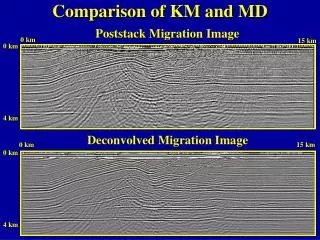
0 km. 0 km. 4 km. 4 km. Comparison of KM and MD. Poststack Migration Image. 0 km. 15 km. Deconvolved Migration Image. 0 km. 15 km. 5. 1. Comparison of RTM and MD Images. RTM. MD. 6. 6. 5. 1. 2. 2. Depth (km). Depth (km). 3. 3. X(km). X(km). X (km). X (km). 10. 10. 8.

E N D
0 km 0 km 4 km 4 km Comparison of KM and MD • Poststack Migration Image • 0 km • 15 km • Deconvolved Migration Image 0 km 15 km
5 • 1 Comparison of RTM and MD Images RTM MD • 6 • 6 • 5 • 1 • 2 • 2 • Depth (km) • Depth (km) • 3 • 3 • X(km) • X(km)
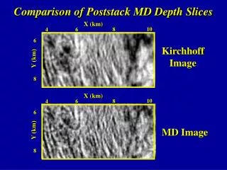
X (km) • X (km) • 10 • 10 • 8 • 8 • 6 • 6 4 4 • 6 • 6 • Y (km) • Y (km) • 8 • 8 Comparison of Poststack MD Depth Slices • Kirchhoff Image • MD Image
Time-Migration Deconvolution Jianxing Hu University of Utah
Outline • Problem • Formation of migration image • Solution • Time-migration deconvolution • Numerical Tests • Synthetic and field data tests • Conclusions
Footprint Amplitude distortion Migration noise and artifacts The Problems • Migration Noise • Recording Footprint • Poor Resolution • Amplitude Distortion • 0 km • 15 km 0 Time (s) 2
Seismograph Source Formation of Migration Image Receivers Point Reflector
Seismograph Migration Response Point Reflector Migration Image
Continue Reflector Migration Image Seismograph Dip Reflection Layer
Migration Response Continue Reflector Migration Image Seismograph Dip Reflection Layer
Outline • Problem • Solution • Numerical Tests • Conclusions
Solution Apply the principle of migration deconvolution to time-migration section
Relation of Migrated Image • and Reflectivity Distribution Model Space where is point scatterer migration response and defined as “migration Green’s function”
Assumption Migration Green’s function is lateral shift invariant: -- 1-D velocity model with an lateral invariant recording geometry and aperture Model Space
Migration Deconvolution Model Space Model Space --- reference position of migration Green’s function
Lateral Velocity Variation • Lateral Velocity Variation • Finite recording geometry Distance Depth
Subdivide the migration image area and use multi- reference migration Green’s function to account for lateral velocity variation and far-field artifacts Multi-Reference migration Green’s function Lateral Velocity Variation
Outline • Problem • Solution • Numerical Tests • Conclusions
Numerical Tests • 2-D SEG/EAGE overthrust model • 2-D Mobil marine data from the North Sea
X (km) 0 0 Time (s) Time (s) 2 2 0 km 15 km KM 0 km 15 km MD
6 6 8 8 10 10 0.5 0.5 1.0 1.0 Zoom Views X (km) X (km) Time (s) KM MD
X (km) 0 0 Time (s) Time (s) 2 2 0 km 15 km KM 0 km 15 km MD
6 6 8 8 10 10 0.5 0.5 1.0 1.0 Zoom Views X (km) X (km) Time (s) KM MD
Numerical Tests • 2-D SEG/EAGE overthrust model • 2-D Mobil marine data from the North Sea
X (km) 0 25 0 Time (s) 4 6 Velocity Model 2500 Velocity (m/s) 1500
X (km) 0 25 0 Time (s) 4 6 Time Migration Image
KM MD 0 Time (s) 4 6 Migration Deconvolution Image X (km) 0 25
KM MD X(km) X(km) 14 14 18 18 2 2 Time (s) Time (s) 2.7 2.7
Spike Decon MD X(km) X(km) 14 14 18 18 2 2 Time (s) Time (s) 2.7 2.7
Whitening Filtering MD X(km) X(km) 14 14 18 18 2 2 Time (s) Time (s) 2.7 2.7
KM MD 0 Time (s) 4 6 Migration Deconvolution Image X (km) 0 25
KM MD X(km) X(km) 10 10 14 14 1 1 Time (s) Time (s) 1.8 1.8
Spike Decon MD X(km) X(km) 10 10 14 14 1 1 Time (s) Time (s) 1.8 1.8
Whitening Filtering MD X(km) X(km) 10 10 14 14 1 1 Time (s) Time (s) 1.8 1.8
KM MD 0 Time (s) 4 6 Migration Deconvolution Image X (km) 0 25
KM MD X(km) X(km) 20 20 24 24 1.5 1.5 Time (s) Time (s) 2.3 2.3
Spike Decon MD X(km) X(km) 20 20 24 24 1.5 1.5 Time (s) Time (s) 2.3 2.3
Whitening Filtering MD X(km) X(km) 20 20 24 24 1.5 1.5 Time (s) Time (s) 2.3 2.3
Outline • Motivation • Solution • Numerical Tests • Conclusions
Works on 2-D synthetic and field poststack time migration data, improve resolution, mitigate some migration artifacts Subdivision method is able to account for lateral-velocity variations and attenuate some far-field artifacts A post-migration processing: Cost 2X Conclusions
Apply time-migration deconvolution to prestack time migration data Future Work Test time-migration deconvolution algorithm on 3D synthetic and field poststack migration data
Acknowledgement I thank the members of Utah Tomography and Modeling /Migration (UTAM) Consortium for their financial support