Download
1 / 55
550 likes | 705 Views
This study presents a detailed comparison between prestack Kirchhoff migration and poststack migration, focusing on the analysis of MD depth slices using North Sea datasets. We explore the methodologies, theoretical foundations, and numerical tests that differentiate these approaches in seismic imaging. The paper outlines the effects of velocity models, reference positions, and depth variations on migrated images, illustrating their relationship with reflectivity distributions. Various numerical tests, including 3D models and datasets, support our findings and conclusions regarding optimal migration strategies.

E N D
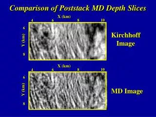
X (km) • X (km) • 10 • 10 • 8 • 8 • 6 • 6 4 4 • 6 • 6 • Y (km) • Y (km) • 8 • 8 Comparison of Poststack MD Depth Slices • Kirchhoff Image • MD Image
4 • 4 • 6 • 6 • 8 • 8 • 10 • 10 • 1 • 1 • Depth (km) • Depth (km) • 4 • 4 Comparison of Prestack Migration and MD Images • X (km) • Prestack Kirchhoff Migration Image of • a North Sea Data Set • X (km) • MD Image
Prestack Migration Deconvolution Jianxing Hu University of Utah
Outline • Methodology • Theory and implementation • Numerical Tests • Synthetic and field data tests • Conclusions
Modeling and Migration Forward Modeling: Model Space Green’s Function Reflectivity Wavelet Seismic data Migration: Data Space Migrated Image Seismic Data
Relation of Migrated Image and Reflectivity Distribution Model Space Where: Data Space Denote as the migration Green’s Function
Reflectivity Modulated by Migration Green’s Function Model Space
Migration Deconvolution Model Space Model Space --- reference position of migration Green’s function
Traveltime Table Migration Green’s function Methodology Calculate migration Green’s function Recording geometry & migrated image dimension + Velocity Model
Apply migration deconvolution filter to the stacked prestack migration image RTM RTM 6 6 5 5 1 1 2 2 Depth (km) Depth (km) 3 3 Offset(km) Offset(km) Methodology Deconvolved Image Migration Image 5 Pseudo-Convolution
Recording Geometry & migrated image dimension + Prestackmigration Green’s function Difference between Poststack MD and Prestack MD Zero-offset trace location & migrated image dimension + Velocity Model Traveltime Table Poststackmigration Green’s function
MD Implementation Entire Migrated Image Cube Division Parts Image Layers Y X Z
MD Scheme for Marine Survey Partitioned Image Cube Smaller Traveltime Table Computing Nodes
MD Scheme for 3-D Land Survey Partitioned Image Cube Smaller Traveltime Table Computing Nodes Problem: Lose Far-Offset Traces
Subdivide the migration image area and use multi- reference migration Green’s function to account for lateral velocity variation and far-field artifacts Multi-Reference migration Green’s function Lateral Velocity Variation
Outline • Methodology • Numerical Tests • Conclusions
Numerical Tests • 3-D point scatterer model • 3-D meandering stream model • 2-D SEG/EAGE overthrust model • 2-D Husky data set (Canadian Foothills) • 3-D SEG/EAGE salt model • 3-D West Texas data set
Recording Geometry 5 X 5 Sources; 21 X 21 Receivers Wavelet frequency 50 Hz (0, 1km) (0, 0) (1km, 1km) (1km, 0) Point scatterer
Prestack KM vs. Prestack MD Y X Y Y X X Y X
Prestack KM vs. Poststack MD Y X Y Y X X Y X
Numerical Tests • 3-D point scatterer model • 3-D meandering stream model • 2-D SEG/EAGE overthrust model • 2-D Husky data set (Canadian Foothills) • 3-D SEG/EAGE salt model • 3-D West Texas data set
Recording Geometry 5 X 5 Sources; 21 X 21 Receivers Wavelet frequency 50 Hz (0, 1 km) (0, 0) (1 km,1 km) (1 km, 0) A river channel
Meandering River Model X (m) 0 1000 0 Depth (m) 1000
X (m) 0 1000 0 Depth (m) 1000 Kirchhoff Migration Image
X (m) 0 1000 0 Depth (m) 1000 MD Image
Numerical Tests • 3-D point scatterer model • 3-D meandering stream model • 2-D SEG/EAGE overthrust model • 2-D Husky data set (Canadian Foothills) • 3-D SEG/EAGE salt model • 3-D West Texas data set
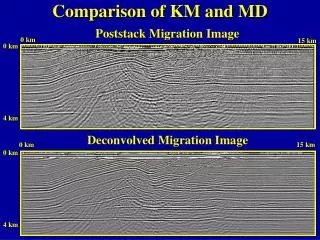
0 km 20 km 0 km 4 km • Prestack Migration Image X(km) 0 km • 20 km 0 km Depth (km) 4 km • Deconvolved Migration Image X(km) Depth (km)
Zoom View of KM and MD 3 3 7 7 X (km) X (km) 2 2 Depth (km) Depth (km) 3 3 4 4 Prestack KM Prestack MD
Numerical Tests • 3-D point scatterer model • 3-D meandering stream model • 2-D SEG/EAGE overthrust model • 2-D Husky data set (Canadian Foothills) • 3-D SEG/EAGE salt model • 3-D West Texas data set
X(km) 10 0 5 0 2 Depth (km) 6 Husky Prestack Migration Image 4
X(km) 10 0 5 0 2 Depth (km) 6 Velocity Model for Husky Data 7000 Velocity (m/s) 3200
X(km) 10 0 5 0 2 Depth (km) 6 MD with 3 reference positions
X(km) 10 0 5 0 2 Depth (km) 6 MD with 20 reference positions
KM Image MD Image 3 references MD Image 20 references
X(km) 10 0 5 0 2 Depth (km) 6 MD with 20 reference positions A
5 9 X(km) 1 KM Depth (km) 3 5 X(km) 9 1 MD Depth (km) 3
X(km) 10 0 5 0 2 Depth (km) 6 MD with 20 reference positions B
11 14 X(km) 1 KM Depth (km) 3 11 X(km) 14 1 MD Depth (km) 3
X(km) 10 0 5 0 2 Depth (km) 6 MD with 20 reference positions C
10 X(km) 14 2 KM Depth (km) 5 10 X(km) 14 2 MD Depth (km) 5
10 X(km) 14 2 KM Depth (km) Whitening & Bandpass 5 10 X(km) 14 2 MD Depth (km) 5
Numerical Tests • 3-D point scatterer model • 3-D meandering stream model • 2-D SEG/EAGE overthrust model • 2-D Husky data set • 3-D SEG/EAGE salt model • 3-D West Texas data set
Y (km) 5 8 0 0 Depth (km) 2 2 4 4 Y (km) 5 8 KM Inline (97,Y) Section MD Inline (97,Y) Section
X (km) X (km) 8 8 11 11 0 0 2 2 4 4 Depth (km) KM Crossline (X,97) Section MD Crossline (X,97) Section
Depth Slices Y (km) Y (km) 5 5 8 8 8 8 X (km) X (km) 11 11 KM MD Y (km) 5 8 Y (km) 5 8 8 8 600 m X (km) X (km) 11 11 800 m
Numerical Tests • 3-D point scatterer model • 3-D meandering stream model • 2-D SEG/EAGE overthrust model • 2-D Husky data set • 3-D SEG/EAGE salt model • 3-D West Texas data set
Velocity Model for West Texas Data X (kft) 0 15 0 20 Velocity (kft/s) Depth(kft) 14 6
West Texas Data X (kft) 0 10 4 8 Depth (kft) KM Inline Section (X,93) 12 16
X (kft) 0 10 4 8 Depth (kft) 12 16 West Texas Data KM Crossline Section (93,Y)