Bayes Classifiers and Generative Methods
Bayes Classifiers and Generative Methods. CSE 4309 – Machine Learning Vassilis Athitsos Computer Science and Engineering Department University of Texas at Arlington. The Stages of Supervised Learning. To build a supervised learning system, we must implement two distinct stages.

Bayes Classifiers and Generative Methods
E N D
Presentation Transcript
Bayes Classifiers and Generative Methods CSE 4309 – Machine Learning VassilisAthitsos Computer Science and Engineering Department University of Texas at Arlington
The Stages of Supervised Learning • To build a supervised learning system, we must implement two distinct stages. • The training stage is the stage where the system uses training data to learn a model of the data. • The decision stage is the stage where the system is given new inputs (not included in the training data), and the system has to decide the appropriate output for each of those inputs. • The problem of deciding the appropriate output for an input is called the decision problem.
The Bayes Classifier • Let X be the input space for some classification problem. • Suppose that we have a function p(x | Ck) that produces the conditional probability of any x in X given any class label Ck. • Suppose that we also know the prior probabilities p(Ck) of all classes Ck. • Given this information, we can build the optimal (most accurate possible) classifier for our problem. • We can prove that no other classifier can do better. • This optimal classifier is called the Bayes classifier.
The Bayes Classifier • So, how do we define this optimal classifier? Let's call it B. • B(x) = ??? • Any ideas?
The Bayes Classifier • First, for every class Ck, compute p(Ck| x) using Bayes rule. • To compute the above, we need to compute p(x). How can we compute p(x)?
The Bayes Classifier • First, for every class Ck, compute p(Ck| x) using Bayes rule. • To compute the above, we need to compute p(x). How can we compute p(x)? • By applying the sum rule: • Let be the set of all possible classes.
The Bayes Classifier • Using , we can now define the optimal classifier: • Can anyone try to guess?
The Bayes Classifier • Using , we can now define the optimal classifier: • What does this mean? What is ? • It is the class c that maximizes p(Ck| x).
The Bayes Classifier • Using , we can now define the optimal classifier: • B(x) is called the Bayes Classifier. • It is the most accurate classifier you can possibly get.
The Bayes Classifier • Using , we can now define the optimal classifier: • B(x) is called the Bayes Classifier. • Important note: the above formulas can also be applied when P(x | c) is a probability density function.
Bayes Classifier Optimality • Why is this a reasonable definition for B(x)? • Why is it the best possible classifier? • ???
Bayes Classifier Optimality • Why is this a reasonable definition for B(x)? • Why is it the best possible classifier? • Because B(x) provides the answer that is most likely to be true. • When we are not sure what the correct answer is, our best bet is the answer that is the most likely to be true.
Bayes Classifier in the Boxes and Fruits Example • Quick review of the boxes and fruits example: • We have two boxes. • A red box, that contains two apples and six oranges. • A blue box, that contains three apples and one orange. • An experiment is conducted as follows: • We randomly pick a box. • We pick the red box 40% of the time. • We pick the blue box 60% of the time. • We randomly pick up one item from the box. • All items are equally likely to be picked. • We put the item back in the box.
Bayes Classifier for Boxes and Fruits: Learning Stage • Input: F, the type of fruit. • Output: B, the type of box from which F was picked. • Learning stage: compute p(F | B), for all combinations of F and B. • How do we compute p(F | B)? Suppose someone has given us one million training examples (Fi, Bi), where Fi was a fruit that was picked, and Bi was the box that Fi was picked from. • We then use the frequentist approach, to compute: • p(F = a | B = r), p(F = o | B = r), p(F = a | B = b), p(F = o | B = b) • How do we compute those?
Bayes Classifier for Boxes and Fruits: Learning Stage • Training data: (F1, B1), (F2, B2), …, (F1000000, B1000000). • In other words: to compute the probability that the fruit is an apple given that the box is red, we compute the ratio where: • The numerator is the number of training examples where the fruit was an apple and the box was red. • The denominator is the number of training examples where the box was red.
Bayes Classifier for Boxes and Fruits: Learning Stage • This way, we can compute p(F = a | B = r), p(F = o | B = r), p(F = a | B = b), p(F = o | B = b) • Suppose that we got very lucky, and the probabilities we computed are actually the correct ones: • p(F = a | B = r) = 2/8. • p(F = o | B = r) = 6/8. • p(F = a | B = b) = 3/4. • p(F = o | B = b) = 1/4. • In practice, if we have a million examples for this problem, we will almost certainly estimate probabilities extremely close to the correct ones.
Bayes Classifier for Boxes and Fruits: Decision Stage • We got a fruit F, and it is an apple. • What box did F come from? • How do we determine that using a Bayes classifier? • We must compute p(B = r | F = a) and p(B = b | F = a), and see which one is larger.
Bayes Classifier for Boxes and Fruits: Decision Stage • So, we have computed: • What does the Bayes classifier output for F=a? • The output is that B=b, because that gives the highest posterior.
Bayes Classifier Limitations • Will a Bayes classifier always have perfect accuracy?
Bayes Classifier Limitations • Will a Bayes classifier always have perfect accuracy? • No. For example: • As we just saw, when the fruit is an apple, the classifier will always predict that the box was the blue one. • However, there will be times when the box is the red one. • In those cases, the output will be incorrect. • However, no other classifier can do any better in that case. • Any classifier, has to give a fixed prediction (either B=r or B=b) for F=a. • If the prediction is that B=b, it will be correct 81.81% of the time. • If the prediction is that B=r, it will be correct 18.18% of the time. • Obviously, the Bayes classifier produces predictions that give the best possible classification accuracy.
Bayes Classifier Limitations • So, we know the formula for the optimal classifier for any classification problem. • Why don't we always use the Bayes classifier? • Why are we going to study other classification methods in this class? • Why are people still trying to come up with new classification methods, if we already know that none of them can beat the Bayes classifier?
Bayes Classifier Limitations • So, we know the formula for the optimal classifier for any classification problem. • Why don't we always use the Bayes classifier? • Why are we going to study other classification methods in this class? • Why are researchers still trying to come up with new classification methods, if we already know that none of them can beat the Bayes classifier? • Because, sadly, the Bayes classifier has a catch. • To construct the Bayes classifier, we need to compute P(x | c), for every x and every c. • In most cases, we cannot compute P(x | c) precisely enough.
An Example: Recognizing Faces • As an example of how difficult it can be to estimate probabilities, let's consider the problem of recognizing faces in 100x100 images. • Suppose that we want to build a Bayesian classifier B(x) that estimates, given a 100x100 image x, whether x is a photograph of Michael Jordan or Kobe Bryant. • Input space: the space of 100x100 color images. • Output space: {Jordan, Bryant}. • We need to compute: • P(x | Jordan). • P(x | Bryant). • How feasible is that? • To answer this question, we must understand how images are represented mathematically.
Images • An image is a 2D array of pixels. • In a color image, each pixel is a 3-dimensional vector, specifying the color of that pixel. • To specify a color, we need three values (r, g, b): • r specifies how "red" the color is. • g specifies how "green" the color is. • b specifies how "blue" the color is. • Each value is a number between 0 and 255 (an 8-bit unsigned integer). • So, a color image is a 3D array, of size rows x cols x 3.
RGB Values and Colors • Each pixel contains three integer values: R, G, B. • The red, green, and blue values of the color of the pixel. • Each value is between 0 and 255. • Each value can be stored as an 8-bit unsigned integer. • Here are some example RGB values and their associated colors: R = 200G = 0 B = 0 R = 0G = 200 B = 0 R = 0G = 0 B = 200 R = 200G = 100 B = 50 R = 152G = 24 B = 210 R = 200G = 200 B = 100
Images as Vectors • Suppose we have a color image, with R rows and C columns. • Then, that image is specified using R*C*3 numbers. • The image is represented as a vector, whose number of dimensions is R*C*3. • If the image is grayscale, then we "only" need R*C dimensions. • Either way, the number of dimensions is huge. • For a small 100x100 color image, we have 30,000 dimensions. • For an 1920x1080 image (the standard size for HD movies these days), we have 6,220,800 dimensions.
Estimating Probabilities of Images • We want a classifier B(x) that estimates, given a 100x100 image x, whether x is a photograph of Michael Jordan or Kobe Bryant. • Input space: the space of 100x100 color images. • Output space: {Jordan, Bryant}. • We need to compute: • P(x | Jordan). • P(x | Bryant). • P(x | Jordan) is a joint distribution of 30,000 real-valued variables. • Each variable has 256 possible values. • We need to compute and store 25630,000numbers. • We have neither enough storage to store so many numbers, nor enough training data to compute all these values.
Generative Methods • Supervised learning methods are divided into generative methods and discriminative methods. • Generative methods: • Learning stage: use the training data to estimate class-conditional probabilities p(x | Ck), where x is an element of the input space, and Ckis a class label (i.e., Ck is an element of the output space). • Decision stage: given an input x: • Use Bayes rule to compute P(Ck | x) for every possible output Ck. • Output the Ck that gives the highest P(Ck | x). • Generative methods use the Bayes classifier at decision stage.
Discriminative Methods • Discriminative methods: • Learning stage: use the training data to learn a discriminant function f(x), that directly maps inputs to class labels. • Decision stage: given input x, output f(x). • Discriminative methods do not need to learn p(x | Ck). • In many cases, p(x | Ck) is too complicated, and it requires too many resources (training data, computation time) to learn p(x | Ck) accurately. • In such cases, discriminative methods are a more realistic alternative.
Options when Accurate Probabilities are Unknown • In pattern classification problems, our data is oftentimes too complex to allow us to compute probability distributions precisely. • So, what can we do? • ???
Options when Accurate Probabilities are Unknown • In pattern classification problems, our data is oftentimes too complex to allow us to compute probability distributions precisely. • So, what can we do? • We have two options. • One is to not use a Bayes classifier, and instead use a discriminative method. • We will study several such methods, such as neural networks, decision trees, support vector machines.
Options when Accurate Probabilities are Unknown • The second option is to still use a Bayes classifier, and estimate approximate probabilities p(x | Ck). • In an approximate method, we do not aim to find the true underlying probability distributions. • Instead, approximate methods are designed to require reasonable memory and reasonable amounts of training data, so that we can actually use them in practice.
Bayes and “pseudo-Bayes” Classifiers • This approach is very common in classification: • Estimate probability distributions P(x | Ck), using an approximate method. • Use the Bayes classifier approach and output, given x, • The resulting classifier looks like a Bayes classifier, but is not a true Bayes classifier. • It is not necessarily the most accurate classifier we can possibly get, because the probabilities are not necessarily correct. • The true Bayes classifier uses the true probabilities P(x | c).
Approximate Probability Estimation • Our next topic will be to look at some popular approximate methods for estimating probability distributions. • Histograms. • Gaussians (we have already discussed this). • Mixtures of Gaussians.
The Naïve Bayes Classifier • The naïve Bayes classifier is a method that makes the (typically unrealistic) assumption that the different dimensions of an input vector are independent of each othergiven the class. • The naïve Bayes classifier can be combined with pretty much any probability estimation method, such as Gaussians. • The naïve Bayes approach greatly simplifies probability calculations. • Instead of computing complicated high-dimensional probability functions (or probability density functions) p(X1, …, Xd | Ck): • We compute a separate probability (or density) for each dimension: pi(X | Ck). • Probabilities of high-dimensional vectors are simply the products of 1D probabilities:
The Naïve Bayes Classifier • Example: Suppose inputs come from a 100-dimensional space: X = (X1, …, X100). • If we wanted to estimate a 100-dimensional Gaussian, we would need to estimate: • 100 numbers for the mean. • About 5000 numbers for the covariance matrix. • Using the naïve Bayes approach. • We compute a separate Gaussian for each dimension. • So, in total, we compute 100 separate Gaussians. • We need to compute 100 means and 100 standard deviations, which is 200 numbers in total.