Bayes classifiers
Bayes classifiers. Edgar Acuna. DT. Input Attributes. Prediction of categorical output. Classifier. Bayes Classifiers. A formidable and sworn enemy of decision trees. BC. How to build a Bayes Classifier.

Bayes classifiers
E N D
Presentation Transcript
Bayes classifiers Edgar Acuna
DT Input Attributes Prediction of categorical output Classifier Bayes Classifiers • A formidable and sworn enemy of decision trees BC
How to build a Bayes Classifier • Assume you want to predict output Y which has arity nY and values v1, v2, … vny. • Assume there are m input attributes called X1, X2, … Xm • Break dataset into nY smaller datasets called DS1, DS2, … DSny. • Define DSi = Records in which Y=vi • For each DSi , learn Density Estimator Mi to model the input distribution among the Y=vi records.
How to build a Bayes Classifier • Assume you want to predict output Y which has arity nY and values v1, v2, … vny. • Assume there are m input attributes called X1, X2, … Xm • Break dataset into nY smaller datasets called DS1, DS2, … DSny. • Define DSi = Records in which Y=vi • For each DSi , learn Density Estimator Mi to model the input distribution among the Y=vi records. • Mi estimates P(X1, X2, … Xm | Y=vi )
How to build a Bayes Classifier • Assume you want to predict output Y which has arity nY and values v1, v2, … vny. • Assume there are m input attributes called X1, X2, … Xm • Break dataset into nY smaller datasets called DS1, DS2, … DSny. • Define DSi = Records in which Y=vi • For each DSi , learn Density Estimator Mi to model the input distribution among the Y=vi records. • Mi estimates P(X1, X2, … Xm | Y=vi ) • Idea: When a new set of input values (X1= u1, X2= u2, …. Xm= um) come along to be evaluated predict the value of Y that makes P(X1, X2, … Xm | Y=vi ) most likely Is this a good idea?
How to build a Bayes Classifier This is a Maximum Likelihood classifier. It can get silly if some Ys are very unlikely • Assume you want to predict output Y which has arity nY and values v1, v2, … vny. • Assume there are m input attributes called X1, X2, … Xm • Break dataset into nY smaller datasets called DS1, DS2, … DSny. • Define DSi = Records in which Y=vi • For each DSi , learn Density Estimator Mi to model the input distribution among the Y=vi records. • Mi estimates P(X1, X2, … Xm | Y=vi ) • Idea: When a new set of input values (X1= u1, X2= u2, …. Xm= um) come along to be evaluated predict the value of Y that makes P(X1, X2, … Xm | Y=vi ) most likely Is this a good idea?
How to build a Bayes Classifier Much Better Idea • Assume you want to predict output Y which has arity nY and values v1, v2, … vny. • Assume there are m input attributes called X1, X2, … Xm • Break dataset into nY smaller datasets called DS1, DS2, … DSny. • Define DSi = Records in which Y=vi • For each DSi , learn Density Estimator Mi to model the input distribution among the Y=vi records. • Mi estimates P(X1, X2, … Xm | Y=vi ) • Idea: When a new set of input values (X1= u1, X2= u2, …. Xm= um) come along to be evaluated predict the value of Y that makes P(Y=vi| X1, X2, … Xm) most likely Is this a good idea?
Terminology • MLE (Maximum Likelihood Estimator): • MAP (Maximum A-Posteriori Estimator):
Bayes Classifiers in a nutshell 1. Learn the distribution over inputs for each value Y. 2. This gives P(X1, X2, … Xm | Y=vi ). 3. Estimate P(Y=vi ). as fraction of records with Y=vi . 4. For a new prediction:
Bayes Classifiers in a nutshell 1. Learn the distribution over inputs for each value Y. 2. This gives P(X1, X2, … Xm | Y=vi ). 3. Estimate P(Y=vi ). as fraction of records with Y=vi . 4. For a new prediction: • We can use our favorite Density Estimator here. • Right now we have two options: • Joint Density Estimator • Naïve Density Estimator
Joint Density Bayes Classifier In the case of the joint Bayes Classifier this degenerates to a very simple rule: Ypredict= the class containing most records in which X1= u1, X2= u2, …. Xm= um. Note that if no records have the exact set of inputs X1= u1, X2= u2, …. Xm= um, then P(X1, X2, … Xm | Y=vi ) = 0 for all values of Y. In that case we just have to guess Y’s value
Ejemplo: Continuacion X1=0,X2=0, x3=1 sera asignado a la clase 1 . Notar tambien que en esta clase el record (0,0,1) aparece mas veces que en la clase 0.
Naïve Bayes Classifier In the case of the naive Bayes Classifier this can be simplified:
Naïve Bayes Classifier In the case of the naive Bayes Classifier this can be simplified: Technical Hint: If you have 10,000 input attributes that product will underflow in floating point math. You should use logs:
Ejemplo: Continuacion X1=0,X2=0, x3=1 sera asignado a la clase 1
BC Results: “XOR” The “XOR” dataset consists of 40,000 records and 2 Boolean inputs called a and b, generated 50-50 randomly as 0 or 1. c (output) = a XOR b The Classifier learned by “Joint BC” The Classifier learned by “Naive BC”
BC Results: “MPG”: 392 records The Classifier learned by “Naive BC”
More Facts About Bayes Classifiers • Many other density estimators can be slotted in*. • Density estimation can be performed with real-valued inputs* • Bayes Classifiers can be built with real-valued inputs* • Rather Technical Complaint: Bayes Classifiers don’t try to be maximally discriminative---they merely try to honestly model what’s going on* • Zero probabilities are painful for Joint and Naïve. A hack (justifiable with the magic words “Dirichlet Prior”) can help*. • Naïve Bayes is wonderfully cheap. And survives 10,000 attributes cheerfully! *See future Andrew Lectures
Naïve Bayes classifier Naïve Bayes classifier puede ser aplicado cuando hay predictoras continuas, pero hay que aplicar previamente un metodo de discretizacion tal como: Usando intervalos de igual ancho, usando intervalos con igual frecuencia, ChiMerge,1R, Discretizacion usando el metodo de la entropia con distintos criterios de parada, Todos ellos estan disponible en la libreria dprep( ver disc.mentr, disc.ew, disc.ef, etc) . La libreria e1071 de R contiene una funcion naiveBayes que calcula el clasificador naïve Bayes. Si la variable es continua asume que sigue una distribucion Gaussiana.
The misclassification error rate The misclassification error rate R(d) is the probability that the classifier d classifies incorrectly an instance coming from a sample (test sample) obtained in a later stage than the training sample. Also is called the True error or the actual error. It is an unknown value that needs to be estimated.
Methods for estimation of the misclassification error rate • Resubstitution or Aparent Error (Smith, 1947). This is merely the proportion of instances in the training sample that are incorrectly classified by the classification rule. In general is an estimator too optimistic and it can lead to wrong conclusions if the number of instances is not large compared with the number of features. This estimator has a large bias. • ii) “Leave one out” estimation. (Lachenbruch, 1965). In this case an instance is omitted from the training sample. Then the classifier is built and the prediction for the omitted instances is obtained. One must register if the instance was correctly or incorrectly classfied. The process is repeated for all the instances in the training sample and the estimation of the ME will be given by the proportion of instances incorrectly classified. This estimator has low bias but its variance tends to be large.
Methods for estimation of the misclassification error rate iii) Cross validation. (Stone, 1974) In this case the training sample is randomly divided in v parts (v=10 is the most used). Then the classifier is built using all the parts but one. The omitted part is considered as the test sample and the predictions for each instance on it are found. The CV misclassification error rate is found by adding the misclassification on each part and dividing them by the total number of instances. The CV estimated has low bias but high variance. In order to reduce the variability we usually repeat the estimation several times. The estimation of the variance is a hard problem (bengio and Grandvalet, 2004).
Methods for estimation of the misclassification error rate iv) The holdout method. A percentage (70%) of the dataset is considered as the training sample and the remaining as the test sample. The classifier is evaluated in the test sample. The experiment is repeated several times and then the average is taken. v) Bootstrapping. (Efron, 1983). In this method we generate several training samples by sampling with replacement from the original training sample. The idea is to reduce the bias of the resubstitution error. It is almost unbiased, but it has a large variance. Its computation cost is high. There exist several variants of this method.
Naive Bayes para Bupa Sin discretizar > a=naiveBayes(V7~.,data=bupa) > pred=predict(a,bupa[,-7],type="raw") > pred1=max.col(pred) > table(pred1,bupa[,7]) pred1 1 2 1 112 119 2 33 81 > error=152/345 [1] 0.4405797 Discretizando con el metodo de la entropia > dbupa=disc.mentr(bupa,1:7) > b=naiveBayes(V7~.,data=dbupa) > pred=predict(b,dbupa[,-7]) > table(pred,dbupa[,7]) pred 1 2 1 79 61 2 66 139 > error1=127/345 [1] 0.3681159
Naïve Bayes para Diabetes Sin Descritizar > a=naiveBayes(V9~.,data=diabetes) > pred=predict(a,diabetes[,-9],type="raw") > pred1=max.col(pred) > table(pred1,diabetes[,9]) pred1 1 2 1 421 104 2 79 164 > error=(79+104)/768 [1] 0.2382813 Discretizando > ddiabetes=disc.mentr(diabetes,1:9) > b=naiveBayes(V9~.,data=ddiabetes) > pred=predict(b,ddiabetes[,-9]) > table(pred,ddiabetes[,9]) pred 1 2 1 418 84 2 82 184 > 166/768 [1] 0.2161458
Naïve Bayes usando discretizacion ChiMerge > chibupa=chiMerge(bupa,1:6) > b=naiveBayes(V7~.,data=chibupa) > pred=predict(b,chibupa[,-7]) > table(pred,chibupa[,7]) pred 1 2 1 117 21 2 28 179 > error=49/345 [1] 0.1420290 > chidiab=chiMerge(diabetes,1:8) > b=naiveBayes(V9~.,data=chidiab) > pred=predict(b,chidiab[,-9]) > table(pred,chidiab[,9]) pred 1 2 1 457 33 2 43 235 > error=76/768 [1] 0.09895833
Otros clasificadores Bayesianos Analisis Discriminante Lineal (LDA). Aqui se asume que la funcion de clase condicional P(X1,…Xm/Y=vj) se asume que es normal multivariada para cada vj. Se supone ademas que la matriz de covarianza es igual para cada una de las clases. La regla de decision para asignar el objeto x se reduce a Notar que la regla de decision es lineal en el vector de predictoras x. Estrictamente hablando solo deberia aplicarse cuando las predictoras son continuas.
Ejemplos de LDA:Bupa y Diabetes > bupalda=lda(V7~.,data=bupa) > pred=predict(bupalda,bupa[,-7])$class > table(pred,bupa[,7]) pred 1 2 1 78 35 2 67 165 > error=102/345 [1] 0.2956522 > diabeteslda=lda(V9~.,data=diabetes) > pred=predict(diabeteslda,diabetes[,-9])$class > table(pred,diabetes[,9]) pred 1 2 1 446 112 2 54 156 > error=166/768 [1] 0.2161458
Otros clasificadores Bayesianos Los k vecinos mas cercanos : (k nearest neighbor). Aqui la funcion de clase condicional P(X1,…Xm/Y=vj) es estimada por el metodo de los k-vecinos mas cercanos. Estimadores basados en estimacion de densidad por Kernel. Estimadores basados en estimacion de la densidad condiiconal usando mezclas Gaussianas
El clasificador k-nn • En el caso multivariado, el estimado de la función de densidad tiene la forma donde vk(x) es el volumen de un elipsoide centrado en x de radio rk(x), que a su vez es la distancia de x al k-ésimo punto más cercano.
El clasificador k-nn Desde el punto de vista de clasificacion supervisada el método k-nn es bien simple de aplicar. En efecto, si las funciones de densidades condicionales f(x/Ci) de la clase Ci que aparecen en la ecuación son estimadas por k-nn. Entonces, para clasificar un objeto, con mediciones dadas por el vector x, en la clase Ci se debe cumplir que para ji. Donde ki y kj son los k vecinos de x que caen en las clase Ci y Cj respectivamente.
El clasificador k-nn Asumiendo priors proporcionales a los tamaños de las clases (ni/n y nj/n respectivamente) lo anterior es equivalente a: ki>kj para jiLuego, el procedimiento de clasificación sería así: 1) Hallar los k objetos que están a una distancia más cercana al ojbeto x, k usualmente es un número impar 1 o 3. 2) Si la mayoría de esos k objetos pertenecen a la clase Ci entonces el objeto x es asignado a ella. En caso de empate se clasifica al azar.
El clasificador k-nn Hay dos problemas en el método k-nn, la elección de la distancia o métrica y la elección de k. • La métrica más elemental que se puede elegir es la euclideana d(x,y)=(x-y)'(x-y). Esta métrica sin embargo, puede causar problemas si las variables predictoras han sido medidas en unidades muy distintas entre sí. Algunos prefieren rescalar los datos antes de aplicar el método. Otra distancia bien usada es la distancia Manhatan definida por d(x,y)=|x-y|. Hay metricas especiales cuando hay distintode variables en el conjunto de datos. • Enas y Choi (1996) usando simulación hicieron un estudio para determinar el k óptimo cuando solo hay dos clases presentesy determinaron que si los tamaños muestrales de las dos clases son comparables entonces k=n3/8 si habia poca diferencia entre las matrices de covarianzas de los grupos y k=n2/8 si habia bastante diferencia entre las matrices de covarianzas.
Ejemplo de knn: Bupa > bupak1=knn(bupa[,-7],bupa[,-7],as.factor(bupa[,7]),k=1) > table(bupak1,bupa[,7]) bupak1 1 2 1 145 0 2 0 200 error=0% > bupak3=knn(bupa[,-7],bupa[,-7],as.factor(bupa[,7]),k=3) > table(bupak3,bupa[,7]) bupak3 1 2 1 106 29 2 39 171 error=19.71% > bupak5=knn(bupa[,-7],bupa[,-7],as.factor(bupa[,7]),k=5) > table(bupak5,bupa[,7]) bupak5 1 2 1 94 23 2 51 177 error=21.44%
Ejemplo de knn: diabetes > diabk3=knn(diabetes[,-9],diabetes[,-9],as.factor(diabetes[,9]),k=3) > table(diabk3,diabetes[,9]) diabk1 1 2 1 459 67 2 41 201 error=14.06% > diabk5=knn(diabetes[,-9],diabetes[,-9],as.factor(diabetes[,9]),k=5) > table(diabk5,diabetes[,9]) diabk1 1 2 1 442 93 2 58 175 error=19.66
What you should know • Bayes Classifiers • How to build one • How to predict with a BC • How to estimate the misclassification error.