Download
1 / 2
20 likes | 39 Views
The Bayes methods are popular in classification because they are optimal. To apply Bayes methods, it is required that prior probabilities and distribution of patterns for class should be known. The pattern is assigned to highest posterior probability class. The three main methods under Bayes classifier are Byes theorem, the Naive Bayes classifier and Bayesian belief networks. Harshad M. Kubade "The Overview of Bayes Classification Methods" Published in International Journal of Trend in Scientific Research and Development (ijtsrd), ISSN: 2456-6470, Volume-2 | Issue-4 , June 2018, URL: https://www.ijtsrd.com/papers/ijtsrd15750.pdf Paper URL: http://www.ijtsrd.com/computer-science/data-miining/15750/the-overview-of-bayes-classification-methods/harshad-m-kubade<br>

E N D
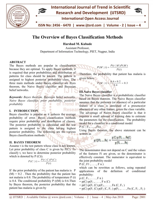
International Research Research and Development (IJTSRD) International Open Access Journal verview of Bayes Classification Methods International Journal of Trend in Scientific Scientific (IJTSRD) International Open Access Journal ISSN No: 2456 ISSN No: 2456 - 6470 | www.ijtsrd.com | Volume 6470 | www.ijtsrd.com | Volume - 2 | Issue – 4 The Overview of Bayes Classification ethods Harshad M. Kubade Assistant Professor, Department of Information Department of Information Technology, PIET, Nagpur, India ABSTRACT The Bayes methods are popular in classification because they are optimal. To apply Bayes methods, it is required that prior probabilities and distribution of patterns for class should be known. The pattern is assigned to highest posterior probability class. The three main methods under Bayes classifier are Byes theorem, the Naive Bayes classifier and Bayesian belief networks. Keywords: Bayes theorem, Bayesian belief networks, Naive Bayes classifier, prior probability, posterior probability I.INTRODUCTION Bayes classifier is popular as it reduces the average probability of error. Bayes classification methods require prior probability and distribution of classes. The posterior probability is calculated and the test pattern is assigned to the class having highest posterior probability. The following are the various Bayes classification methods. II. BAYES THEOREM Assume t is the test pattern whose class is not known. Let prior probability of class C is given by P(C). To classify t, we have to determine posterior probability which is denoted by P (C|t). P t C P The Bayes methods are popular in classification P ( t | M ) t P ( M ) P ( M | t ) apply Bayes methods, it P ( ) is required that prior probabilities and distribution of patterns for class should be known. The pattern is assigned to highest posterior probability class. The three main methods under Bayes classifier are Byes ayes classifier and Bayesian Therefore, the probability that patient has malaria is Therefore, the probability that patient has malaria is given below 6 . 0 ) | ( t M P 4 . 2 . 0 3 . 0 . 0 III. Naive Bayes classifier The Naive Bayes classifier is a probabilistic classifier based on Bayes theorem. The Naive Bayes classifier assumes that the presence (or absence) of a particular feature of a class is unrelated of a presence(or absence) of any other feature, given the cla The advantage of Naive Bayes classifier is that it requires a small amount of training data to estimate the parameters for the classification. The probability model for a classifier is a conditional model P (C | F1, ....., Fn) Using Bayes theorem, the above statement can be written as The Naive Bayes classifier is a probabilistic classifier based on Bayes theorem. The Naive Bayes classifier assumes that the presence (or absence) of a particular feature of a class is unrelated of a presence(or absence) of any other feature, given the class variable. The advantage of Naive Bayes classifier is that it requires a small amount of training data to estimate the parameters for the classification. The probability model for a classifier is a conditional model Bayes theorem, Bayesian belief networks, Naive Bayes classifier, prior probability, posterior Bayes classifier is popular as it reduces the average Bayes classification methods require prior probability and distribution of classes. The posterior probability is calculated and the test pattern is assigned to the class having highest posterior probability. The following are the various heorem, the above statement can be Assume t is the test pattern whose class is not known. Let prior probability of class C is given by P(C). To classify t, we have to determine posterior probability The denominator does not depend on C and the values of the features Fi are given, so the denominator is effectively constant. The numerator is equivalent to the joint probability model P (C, F1 , . . . , F n ) which can be rewritten as follows, using repeated applications of the definition probability: p (C, F1 , . . . , F n ) = p(C) p(F1 , . . . , F n |C) = p(C) p(F1 |C) p(F2 , . . . , Fn |C, F = p(C) p(F1 |C) p(F2 |C, F1 ) p(F ) p(F3 , . . . , Fn |C, F1 , F2 ) The denominator does not depend on C and the values of the features Fi are given, so the denominator is effectively constant. The numerator is equivalent to ( t | C ) t P ( C ) ( | ) P ( ) If the prior probability of the patient has malaria is P (M) = 0.2 . Then the probability that the patient has not malaria is 0.8. The probability of temperature P is 0.4. The conditional probability P (t|M) is 0.6.Then by Bayes theorem, the posterior proba patient has malaria is given by which can be rewritten as follows, using repeated applications of the definition of prior probability of the patient has malaria is P (M) = 0.2 . Then the probability that the patient has not malaria is 0.8. The probability of temperature P (t) of conditional conditional (t|M) is 0.6.Then by Bayes theorem, the posterior probability that the , . . . , Fn |C, F1 ) @ IJTSRD | Available Online @ www.ijtsrd.com @ IJTSRD | Available Online @ www.ijtsrd.com | Volume – 2 | Issue – 4 | May-Jun 2018 Jun 2018 Page: 2801
International Journal of Trend in Scientific Research and Development (IJTSRD) ISSN: International Journal of Trend in Scientific Research and Development (IJTSRD) ISSN: International Journal of Trend in Scientific Research and Development (IJTSRD) ISSN: 2456-6470 3.a set of conditional probability distributions giving P(Xi|parents(Xi)). Full joint distribution is defined in terms of local conditional distributions as P(X1, X2, …..., Xn) = i 1 If node Xi has no parents, its local probability distribution is said to be unconditional, otherwise it is conditional. If the value of a node is observed, then the node is said to be an evidence node. Each variable is associated with a conditional probability table which gives the probability of this variabl different values of its parent nodes. The value of P (X1, ..., Xn ) for a particular set of values for the variables can be easily computed from the conditional probability table. Consider the five events M, N, X, Y, and Z. Each event has a conditional probability table. The events M and N are independent events i. e. they are not influenced by any other events. The conditional probability table for X shows the probability of X, probability table for X shows the probability of X, = p(C) p(F1 |C) p(F2 |C, F1 ) p(F3 |C, F1 . , Fn |C, F1 , F2 , F3 ) and so forth. Using independence assumptions, each feature Fi is conditionally independent of every other feature Fj for j ≠ i. This means that p (F i |C, F j ) = p(F i |C) and so the joint model can be expressed as p(C, F1 , . . . , Fn ) = p(C) p(F1 |C) p(F2 · p(Fn |C) =p(C) This means that under the above assumptions of independence, the conditional distribution over the class variable C can be expressed as P(C|1,..Fn)= where Z is a scaling factor dependent only on F Fn , i.e., a constant if the values of the feature variables are known. The naive Bayes classifier combines the Bayes probability model with a decision rule. One common rule is to pick the hypothesis that is most probable; this is known as the maximum a posterior or MAP decision rule. The corresponding classifier is the function ‘‘classify’’ defined as follows: , F2 ) p(F4 , . . probability distributions giving and independence assumptions, each feature Fi is conditionally independent of every other feature Fj for so forth. Using the the naive naive conditional conditional Full joint distribution is defined in terms of local n P(Xi| Parents (Xi)) P(Xi| Parents (Xi)) and so the joint model can be expressed as If node Xi has no parents, its local probability ibution is said to be unconditional, otherwise it is conditional. If the value of a node is observed, then the node is said to be an evidence node. Each variable is associated with a conditional probability table which gives the probability of this variable for different values of its parent nodes. |C) p(F3 |C) · · This means that under the above assumptions of distribution over the The value of P (X1, ..., Xn ) for a particular set of values for the variables can be easily computed from the conditional probability table. where Z is a scaling factor dependent only on F1 , . . , Fn , i.e., a constant if the values of the feature Consider the five events M, N, X, Y, and Z. Each event has a conditional probability table. The events M and N are independent events i. e. they are not influenced by any other events. The conditional The naive Bayes classifier combines the Bayes ability model with a decision rule. One common rule is to pick the hypothesis that is most probable; this is known as the maximum a posterior or MAP decision rule. The corresponding classifier is the IV. Bayesian Belief Network A Bayesian network (or a belief network) is a probabilistic graphical model. This model represents a set of variables and their probabilistic dependencies. Bayesian Belief Networks provide the modeling and reasoning about the uncertainty. Bayesian Belief networks cover both subjective probabilities and probabilities based on objective data. For example, a Bayesian network could represent the probabilistic relationships between diseases and symptoms. Given symptoms, the network can be used to probabilities of the presence of various diseases. A belief network, also called a Bayesian network, is an acyclic directed graph (DAG), where the nodes are random variables. If there is an arc from node A to another node B, A is called a parent of B, and B is a child of A. The set of parent nodes of a node Xi is denoted by its parents (Xi ). Thus, a belief network consists of 1.a DAG, where each node is labeled by a random variable; 2.a domain for each random variable; and a domain for each random variable; and A Bayesian network (or a belief network) is a probabilistic graphical model. This model represents a set of variables and their probabilistic dependencies. Bayesian Belief Networks provide the modeling and Figure: Bayesian Belief Network given the conditions of the events M and N i. e. true or false. The event X occurs if event M is true. The event X also occurs if event N does not occur. The events Y and Z occur if the event X does not occur. figure shows the belief network for the Figure: Bayesian Belief Network given the conditions of the events M and N i. e. true or false. The event X occurs if event M is true. The event X also occurs if event N does not occur. The events Y and Z occur if the event X does not occur. The following figure shows the belief network for the given situation. REFERENCES 1.V Susheela Devi and M Narasimha Murty, “Pattern Recognition: Universities Press (India) Private Limited. Universities Press (India) Private Limited. ayesian Belief networks cover both subjective probabilities and probabilities based on objective data. For example, a Bayesian network could represent the probabilistic relationships between diseases and symptoms. Given symptoms, the network can be used to compute the probabilities of the presence of various diseases. A belief network, also called a Bayesian network, is an acyclic directed graph (DAG), where the nodes are random variables. If there is an arc from node A to V Susheela Devi and M Narasimha Murty, “Pattern Recognition: An An Introduction”, Introduction”, 2.Robert Statistical, Structural And Neural Approaches”, Wiley India (P.) Ltd. Robert Schalkoff, Schalkoff, “Pattern “Pattern And Neural Approaches”, Recognition: Recognition: nt of B, and B is a child of A. The set of parent nodes of a node Xi is denoted by its parents (Xi ). Thus, a belief network 3.Richard O. Duda, Peter E. Hart, David G. Stork, “Pattern Classification”, Wiley India (P.) Ltd. “Pattern Classification”, Wiley India (P.) Ltd. Richard O. Duda, Peter E. Hart, David G. Stork, a DAG, where each node is labeled by a random 4.Bayesian Networks Wikipedia. Bayesian Networks Wikipedia. @ IJTSRD | Available Online @ www.ijtsrd.com | Volume @ IJTSRD | Available Online @ www.ijtsrd.com | Volume – 2 | Issue – 4 | May-Jun 2018 Jun 2018 Page: 2802