Generative and adaptive methods in performance programming
f. . g. p ; q. p | q. p || q. p(q) p<q>. Generative and adaptive methods in performance programming. Paul H J Kelly Imperial College London Joint work with Olav Beckmann Including contributions from Tony Field and numerous students. Where we’re coming from….

Generative and adaptive methods in performance programming
E N D
Presentation Transcript
f g p ; q p | q p || q p(q) p<q> Generative and adaptive methods in performance programming Paul H J Kelly Imperial College London Joint work with Olav Beckmann Including contributions from Tony Field and numerous students
Where we’re coming from… • I lead the Software Performance Optimisation group at Imperial College, London • Stuff I’d love to talk about another time: • Run-time code-motion optimisations across network boundaries in Java RMI • Bounds-checking for C, links with unchecked code • Is Morton-order layout for 2D arrays competitive? • Domain-specific optimisation frameworks • Domain-specific profiling • Proxying in CC-NUMA cache-coherence protocols – adaptive randomisation and combining V & A Science Museum Imperial College Albert Hall Hyde Park
Generative and adaptive methods in performance programming • Performance programming • Performance programming is the discipline of software engineering in its application to achieving performance goals • This talk aims to review a selection of performance programming techniques we have been exploring
Construction • What is the role of constructive methods in performance programming? • “by construction” • “by design” • How can we build performance into a software project? • How can we build-in the means to detect and correct performance problems? • As early as possible • With minimal disruption to the software’s long-term value?
Abstraction • Most performance improvement opportunities come from adapting components to their context • So the art of performance programming is to figure out how to design and compose components so this doesn’t happen • Most performance improvement measures break abstraction boundaries • This talk is about two ideas which can help: • Run-time program generation (and manipulation) • Metadata, characterising data structures, components, and their dependence relationships
Abstraction • Most performance improvement opportunities come from adapting components to their context • So the art of performance programming is to figure out how to design and compose components so this doesn’t happen • Most performance improvement measures break abstraction boundaries • This talk is about two ideas which can help: • Run-time program generation (and manipulation) • Metadata, characterising data structures, components, and their dependence relationships
Abstraction • Most performance improvement opportunities come from adapting components to their context • So the art of performance programming is to figure out how to design and compose components so this doesn’t happen • Most performance improvement measures break abstraction boundaries • This talk is about two ideas which can help: • Run-time program generation (and manipulation) • Metadata, characterising data structures, components, and their dependence relationships
Abstraction • Most performance improvement opportunities come from adapting components to their context • So the art of performance programming is to figure out how to design and compose components so this doesn’t happen • Most performance improvement measures break abstraction boundaries • This talk is about two ideas which can help: • Run-time program generation (and manipulation) • Metadata, characterising data structures, components, and their dependence relationships
Abstraction • This talk: • Communication fusion • Alignment in parallel BLAS • Partial evaluation/specialisation • Adapting to platform/resources • Cross-component loop fusion Adapting to context Dependence metadata Performance metadata Component model to support composition-time adaptation
Adaptation #1: Communication fusion • Example: calculating variance of distributed vector “data” double s1, s2; void sum( double& data ) { double r = 0.0 ; … for (j=jmin;j<=jmax;j++) { r += data[j] ; } MPI_Allreduce(&r,&s1,1,MPI_SUM,...); } void sumsq( double& data ) { double r = 0.0 ; … for (j=jmin;j<=jmax;j++) { r += data[j]*data[j] ; } MPI_Allreduce(&r,&s2,1,...); } Component #1 Component composition double a[…][…],var[…] ; for( i=0; i<N; i++ ) { sum(a[i]) ; sumSq(a[i]) ; var[i] = (s2-s1*s1/N)/(N-1); } Component #2
Adaptation #1: Communication fusion • Example: calculating variance of distributed vector “data” double rVec[2]; void sum( double& data ) { double r = 0.0 ; … for (j=jmin;j<=jmax;j++) { r += data[j] ; } rVec[0] = r; } void sumsq( double& data ) { double r = 0.0 ; … for (j=jmin;j<=jmax;j++) { r += data[j]*data[j] ; } rVec[1]= r; } Component #1 Component composition double a[…][…],var[…] ; for( i=0; i<N; i++ ) { sum(a[i]) ; sumSq(a[i]) ; MPI_Allreduce(&rVec,&s,2, MPI_SUM,..) ; var[i] = (s2-s1*s1/N)/(N-1); } Component #2 • For N=3000 fusing MPI Allreduces improved performance on linux cluster by 48.7%
Adaptation #1: Communication fusion Shared variable declaration CFL_Double s1(0), s2(0) ; void sum( double& data ) { s1 = 0.0 ; … for (j=jmin;j<=jmax;j++) { s1 += data[j] ; } } void sumsq( double& data ) { s2 = 0.0 ; … for (j=jmin;j<=jmax;j++) { s2 += data[j]*data[j] ; } } Component #1 Component composition double a[…][…],var[…] ; for( i=0; i<N; i++ ) { sum(a[i]) ; sumSq(a[i]) ; var[i] = (s2-s1*s1/N)/(N-1); } Global reduction Component #2 Assignment to local force point • For N=3000 our CFL library improved performance on linux cluster by 44.5% Global reduction
Application: ocean plankton ecology model Physics Move Total Biomass computed here Used here Phyto Ocean surface Nutrient Cell Nitrogen computed here Used here Zoo Nz Az Iz CO2z Energy And so on… Stats • 27 reduction operations in total • 3 communications actually required! • 60% speedup for 32-processor AP3000 … Carbon … Evolve A.J. Field, P.H.J. Kelly and T.L. Hansen, "Optimizing Shared Reduction Variables in MPI Programs". In Euro-Par 2002
Adaptation #2: alignment in parallel BLAS • This is a generic conjugate-gradient solver algorithm, part of Dongarra et al’s IML++ library • It is parameterised by the Matrix and Vector types • Our DESOBLAS library implements this API for dense matrices • In parallel using MPI
Adaptation #2: alignment in parallel BLAS • Execution is delayed until output or conditional forces computation • BLAS functions return opaque handles • Library builds up data flow graph “recipe” representing delayed computation • This allows optimization to exploit foreknowledge of how results will be used A r x p:=r q:=A.p :=r.r :=q.p := / • Example: conjugate gradient x:=p+x
Adaptation #2: alignment in parallel BLAS r: blocked row-wise A: blocked row-major x: blocked row-wise A r x p: p:=r q: q and p have incompatible distributions Result of matrix-vector multiply is aligned with the matrix columns Conflict q:=A.p :=r.r :=q.p := / (because result column vector is formed from dot-products across each row) x:=p+x • For parallel dense BLAS, main issue is avoiding unnecessary data redistributions • Consider just the first iteration: Choose default distributions when variables initialised. Vectors are usually replicated
Adaptation #2: alignment in parallel BLAS p: q: x and p have incompatible distributions p: Conflict • We are forced to insert a transpose: r: blocked row-wise A: blocked row-major x: blocked row-wise A r x p:=r q:=A.p transpose :=r.r :=q.p := / x:=p+x
Adaptation #2: alignment in parallel BLAS p: q: p: • We are forced to insert another transpose: A r x p:=r We can transpose either p or x (or we could have kept an untransposed copy of p – if we’d known it would be needed) q:=A.p transpose :=r.r :=q.p transpose := / x:=p+x
Adaptation #2: alignment in parallel BLAS p: q: p: • Delayed execution allows us to see how values will be used and choose better: A r x p:=r If we can foresee how p will be used, we can see it’s the wrong thing to transpose… q:=A.p transpose :=r.r :=q.p transpose := / x:=p+x
Adaptation #2: alignment in parallel BLAS r: blocked row-wise A: blocked row-major x: blocked row-wise Conflict • Delayed execution allows us to see how values will be used and choose better: A r x p:=r If we can foresee how p will be used, we can see it’s the wrong thing to transpose… q:=A.p :=r.r :=q.p := / x:=p+x
Adaptation #2: alignment in parallel BLAS r: blocked row-wise A: blocked row-major x: blocked row-wise • Delayed execution allows us to see how values will be used and choose better: A r x p:=r If we can foresee how p will be used, we can see it’s the wrong thing to transpose… q:=A.p :=r.r transpose :=q.p := / x:=p+x
Avoiding redistributions: performance • Cluster of 2GHz P4, 500 MB RAM, running Linux 2.4.20 and gcc 2.95.3, using C/Fortran bindings (not C++ overloading)
Metadata in DESOBLAS Metadata: affine relationship between operand alignments and result alignment • Each DESOBLAS library operator carries metadata, which is used at run-time to find an optimized execution plan • For optimizing data placement, metadata is set of affine functions relating operator’s output data placement to the placement of each input • Network of invertible linear relationships allows optimizer to shift redistributions around dataflow graph to minimise communication cost • ((broadcasts and reductions involve singular placement relationships - see Beckmann and Kelly, LCPC’99 for how to make this idea still work)) Composition: metadata is assembled according to arcs of data flow graph to define system of alignment constraints: Peter Liniker, Olav Beckmann and Paul H J Kelly, Delayed Evaluation, Self-Optimizing Software Components as a Programming Model. In Euro-Par 2002
Adaptation #3: specialisation #include <TaskGraph> #include <stdio.h> #include <stdlib.h> #include <sys/time.h> using namespace tg; int main( int argc, char argv[] ) { TaskGraph T; int b = 1, c = 1; taskgraph ( T ) { tParameter ( tVar ( int, a ) ); a = a + c; } T.compile ( TaskGraph::GCC ); T.execute ("a", &b, NULL); printf("b = %d\n", b); } • The TaskGraph library is a portable C++ package for building and optimising code on-the-fly • Compare: • `C (tcc) (Dawson Engler) • MetaOCaml (Walid Taha et al) • Jak (Batory, Lofaso, Smaragdakis) • Multi-stage programming: “runtime code generation as a first-class language feature”
Adaptation #3: specialisation #include <TaskGraph> #include <stdio.h> #include <stdlib.h> #include <sys/time.h> using namespace tg; int main( int argc, char argv[] ) { TaskGraph T; int b = 1, c = 1; taskgraph ( T ) { tParameter ( tVar ( int, a ) ); a = a + c; } T.compile ( TaskGraph::GCC ); T.execute ( “a", &b, NULL); printf("b = %d\n", b); } • A taskgraph is an abstract syntax tree for a piece of executable code • Syntactic sugar makes it easy to construct • Defines a simplified sub-language • With first-class multidimensional arrays, no alliasing
Adaptation #3: specialisation #include <TaskGraph> #include <stdio.h> #include <stdlib.h> #include <sys/time.h> using namespace tg; int main( int argc, char argv[] ) { TaskGraph T; int b = 1, c = 1; taskgraph ( T ) { tParameter ( tVar ( int, a ) ); a = a + c; } T.compile ( TaskGraph::GCC ); T.execute (“a", &b, NULL); printf("b = %d\n", b); } • Binding time is determined by types • In this example • c is static • a is dynamic • built using value of c at construction time
Adaptation #3: specialisation void filter (float *mask, unsigned n, unsigned m, const float *input, float *output, unsigned p, unsigned q) { unsigned i, j; int k, l; float sum; int half_n = (n/2); int half_m = (m/2); for (i = half_n; i < p - half_n; i++) { for (j = half_m; j < q - half_m; j++) { sum = 0; for (k = -half_n; k <= half_n; k++) for (l = -half_m; l <= half_m; l++) sum += input[(i + k) * q + (j + l)] * mask[k * n + l]; output[i * q + j] = sum; } } } Better example: • Applying a convolution filter to a 2D image • Each pixel is averaged with neighbouring pixels weighted by a stencil matrix // Loop bounds unknown at compile-time // Trip count 3, does not fill vector registers Mask Image • First without TaskGraph
Adaptation #3: specialisation void taskFilter (TaskGraph &t, float *mask, unsigned n, unsigned m, unsigned p, unsigned q) { taskgraph (t) { unsigned img_size[] = { IMG_SIZE, IMG_SIZE }; tParameter(tArray(float, input, 2, img_size )); tParameter(tArray(float, output, 2, img_size )); unsigned k, l; unsigned half_n = (n/2); unsigned half_m = (m/2); tVar (float, sum); tVar (int, i); tVar (int, j); tFor (i, half_n, p - half_n - 1) { tFor (j, half_m, q - half_m - 1) { sum = 0; for ( k = 0; k < n; ++k ) for ( l = 0; l < m; ++l ) sum += input[(i + k - half_n)][(j + l - half_m)] * mask[k * m + l]; output[i][j] = sum; } } } } • TaskGraph representation of this loop nest • Inner loops are static – executed at construction time • Outer loops are dynamic • Uses of mask array are entirely static • This is deduced from the types of mask, k, m and l. // Inner loops fully unrolled // j loop is now vectorisable • Now with TaskGraph
Adaptation #3: specialisation Image convolution using TaskGraphs: performance • We use a 3x3 averaging filter as convolution matrix • Images are square arrays of single-precision floats ranging in size up to 4096x4096 • Measurements taken on a 1.8GHz Pentium 4-M running Linux 2.4.17, using gcc 2.95.3 and icc 7.0 • Measurements were taken for one pass over the image (Used an earlier release of the TaskGraph library) 2048x2048 big enough 1024x1024 too small
Adaptation #3: specialisation • Application: Sobel filters in image processing (8-bit RGB data) – compared with Intel’s Performance Programming Library
Adaptation #4: Adapting to platform/resources • The TaskGraph library is a tool for dynamic code generation and optimisation • Large performance benefits can be gained from specialisation alone But there’s more: • TaskGraph library builds SUIF intermediate representation • Provides access to SUIF analysis and transformation passes • SUIF (Stanford University Intermediate Form) • Detect and characterise dependences between statements in loop nests • Restructure – tiling, loop fusion, skewing, parallelisation etc
Tiling void taskMatrixMult (TaskGraph &t , TaskLoopIdentifier *loop) { taskgraph ( t ) { tParameter ( tArray ( float, a, 2, sizes ) ); tParameter ( tArray ( float, b, 2, sizes ) ); tParameter ( tArray ( float, c, 2, sizes ) ); tVar ( int, i ); tVar ( int, j ); tVar ( int, k ); tGetId ( loop[0] ); // label tFor ( i, 0, MATRIXSIZE - 1 ) { tGetId ( loop[1] ); // label tFor ( j, 0, MATRIXSIZE - 1 ) { tGetId ( loop[2] ); // label tFor ( k, 0, MATRIXSIZE - 1 ) { c[i][j] += a[i][k] * b[k][j]; } } } } } • Example: matrix multiply int main ( int argc, char **argv ) { TaskGraph mm; TaskLoopIdentifier loop[3]; // Build TaskGraph for ijk multiply taskMatrixMult ( loop, mm ); // Interchange the j and k loops interchangeLoops ( loop[1], loop[2] ); int trip[] = { 64, 64 }; // Tile the j and k loops into 64x64 tiles tileLoop ( 2, &loop[1], trip ); mm.compile ( TaskGraph::GCC ); mm.execute ( "a", a, "b", b, "c", c, NULL ); } Original TaskGraph for matrix multiply Code to interchange and tile
Loop interchange and tiling void taskMatrixMult (TaskGraph &t , TaskLoopIdentifier *loop) { taskgraph ( t ) { tParameter ( tArray ( float, a, 2, sizes ) ); tParameter ( tArray ( float, b, 2, sizes ) ); tParameter ( tArray ( float, c, 2, sizes ) ); tVar ( int, i ); tVar ( int, j ); tVar ( int, k ); tGetId ( loop[0] ); // label tFor ( i, 0, MATRIXSIZE - 1 ) { tGetId ( loop[1] ); // label tFor ( j, 0, MATRIXSIZE - 1 ) { tGetId ( loop[2] ); // label tFor ( k, 0, MATRIXSIZE - 1 ) { c[i][j] += a[i][k] * b[k][j]; } } } } } extern void taskGraph_1(void **params) { float (*a)[512]; float (*b)[512]; float (*c)[512]; int i; int j; int k; int j_tile; int k_tile; a = *params; b = params[1]; c = params[2]; for (i = 0; i <= 511; i++) for (j_tile = 0; j_tile <= 511; j_tile += 64) for (k_tile = 0; k_tile <= 511; k_tile += 64) for (j = j_tile; j <= min(511, 63 + j_tile); j++) for (k = max(0, k_tile); k <= min(511, 63 + k_tile); k++) c[i][k] = c[i][k] + a[i][j] * b[j][k]; } • Generated code (Slightly tidied) Original TaskGraph for matrix multiply int main ( int argc, char **argv ) { TaskGraph mm; TaskLoopIdentifier loop[3]; // Build TaskGraph for ijk multiply taskMatrixMult ( loop, mm ); // Interchange the j and k loops interchangeLoops ( loop[1], loop[2] ); int trip[] = { 64, 64 }; // Tile the j and k loops into 64x64 tiles tileLoop ( 2, &loop[1], trip ); mm.compile ( TaskGraph::GCC ); mm.execute ( "a", a, "b", b, "c", c, NULL ); } Code to interchange and tile
Adaptation #4: Adapting to platform/resources • We can program a search for the best implementation for our particular problem size, on our particular hardware On Pentium 4-M, 1.8 GHz, 512KB L2 cache, 256 MB, running Linux 2.4 and icc 7.1.
Potential for user-directed restructuring • Programmer controls application of sophisticated transformations • Performance benefits can be large – in this example >8x • Different target architectures and problem sizes need different combinations of optimisations • ijk or ikj? • Hierarchical tiling • 2d or 3d? • Copy reused submatrix into contiguous memory? • Matrix multiply is a simple example Olav Beckmann, Alastair Houghton, Paul H J Kelly and Michael Mellor, Run-time code generation in C++ as a foundation for domain-specific optimisation. Domain-Specific Program Generation, Springer (2004).
Cross-component loop fusion • Image processing example • Blur, edge-detection filters then sum with original image • Final two additions using Intel Performance Programming Library:
Cross-component loop fusion • After loop fusion:
Cross-component loop fusion • After loop fusion: • Simple fusion leads to small improvement • Beats Intel library only on large images • Further fusion opportunities require skewing/retiming
Performance-programming Component model U For (i=1; i<N; i++) V[i] = (U[i-1] + U[i+1])/2 Jacobi1D(U,V): V For (i=1; i<N; i++) W[i] = (V[i-1] + V[i+1])/2 Jacobi1D(V,W): W • Dependence metadata • Components should carry a description of their dependence structure • That is based on an abstraction of the component’s Iteration Space Graph (ISG) • Eg to allow simple check for validity of loop and communication fusion • Eg to determine dependence constraints on distribution • Eg so we can align data distributions to minimise communication • To predict communication volumes Fusion invalid: iteration i of second loop reads value generated at iteration i of first loop
Performance-programming Component model • Dependence metadata • Components should carry a description of their dependence structure • That is based on an abstraction of the component’s Iteration Space Graph (ISG) • Eg to allow simple check for validity of loop and communication fusion • Eg to determine dependence constraints on distribution • Eg so we can align data distributions to minimise communication • To predict communication volumes U For (i=1; i<N; i++) V[i] = (U[i-1] + U[i+1])/2 Jacobi1D(U,V): V For (i=1; i<N; i++) W[i] = (V[i-1] + V[i+1])/2 Jacobi1D(V,W): Fusion valid: iteration i of second loop reads value generated at iteration i of first loop W
Performance-programming Component model • Performance metadata • Components should carry a model of how execution time depends on parameters and configuration • That is based on an abstraction of the component’s Iteration Space Graph (ISG) • Eg to allow scheduling and load balancing • Eg to determine communication-computation-recomputation tradeoffs M: Inner loop bounds N: Number of iterations for (it=0; it<N; it++) for (i=1; i<M; i++) V[i] = (U[i-1] + U[i+1])/2 • Output volume: M-1 • Compute volume: N.(M-1) • Input volume: M
Performance-programming Component model • Performance metadata • Components should carry a model of how execution time depends on parameters and configuration • That is based on an abstraction of the component’s Iteration Space Graph (ISG) • Eg to allow scheduling and load balancing • Eg to determine communication-computation-recomputation tradeoffs M: Inner loop bounds N: Number of iterations for (it=0; it<N; it++) for (i=1; i<M; i++) V[i] = (U[i-1] + U[i+1])/2 • Output volume: M-1 • Compute volume: N.(M-1) • Input volume: M
Component metadata research agenda • We want to adapt to shape of data • But in interesting applications, data shape is not regular • Shape description/metadata depends on data values • Metadata size is significant • Metadata generation/manipulation is significant part of computational effort • The problem: • Cost of organising and analysing the data may be large compared to the computation itself • Size of metadata may be large compared with size of the data itself • What does this mean? • Some kind of reflective programming • Arguably, metaprogramming • Programs that make runtime decisions about how much work to do to optimise future execution Paul H J Kelly, Olav Beckmann, Tony Field and Scott Baden, "Themis: Component dependence metadata in adaptive parallel applications". Parallel Processing Letters, Vol. 11, No. 4 (2001)
Conclusions • Performance programming as a software engineering discipline • The challenge of preserving abstractions • The need to design-in the means to solve performance problems • Adaptation to data-flow context • Adaptation to platform/resources • Adaptation to data values, sizes, shapes • Making component composition explicit: build a plan, optimise it, execute it
Acknowledgements • This work was funded by EPSRC • Much of the work was done by colleagues and members of my research group, in particular • Olav Beckmann • Tony Field • Students: • Alastair Houghton, Michael Mellor, Peter Fordham, Peter Liniker, Thomas Hansen