Download
1 / 23
250 likes | 426 Views
Turbulence statistics from DNS and LES - implications for urban canopy models. Omduth Coceal Dept. of Meteorology, Univ. of Reading, UK. Email: o.coceal@reading.ac.uk and Dobre, S.E. Belcher (Reading) T.G. Thomas, Z. Xie, I.P. Castro (Southampton). Interpretation of field experiments.

E N D
Turbulence statistics from DNS and LES - implications for urban canopy models Omduth Coceal Dept. of Meteorology, Univ. of Reading, UK. Email: o.coceal@reading.ac.uk and Dobre, S.E. Belcher (Reading) T.G. Thomas, Z. Xie, I.P. Castro (Southampton)
Interpretation of field experiments Can we hope to understand this … … using this ? • - CFD/LES/DNS can provide detailed spatial information of any statistics • But how realistic are the results? • Compare idealized simulations with less idealized simulations and with field data
Parameterisations & Modelling y h x E.g. Urban canopy models (e.g. Martilli et al., 2002; Coceal & Belcher, 2004 ) • Don’t resolve horizontal heterogeneity at the building/street scale • Take horizontal averages: resolve vertical flow structure Triple decomposition of velocity field Spatial average of Reynolds-averaged momentum equation • CFD can be used to compute these spatially-averaged quantities • How can they be parameterized?
Outline • Description of numerical simulations • Comparisons with wind-tunnel data • Spatially-averaged statistics for different types of building arrays • Regular arrays with different building layouts • Arrays with variable building heights (using results from LES) • Unsteady & organized flow characteristics - comparisons with field data
Direct numerical simulations Coceal et al., BLM (2006) Coceal et al., IJC, to appear (2007) • Parallel LES/DNS code developed by T.G. Thomas • Resolution: 32 x 32 x 32 gridpoints per cube (also 643 gridpoints per cube on a smaller domain) • Total of 512 x 384 x 256 ~50 million gridpoints for large array • Periodic boundary conditions in horizontal; flow driven by constant body force • Largest run took ~3 weeks on 124 processors on SGI Altix
Instantaneous windvectors in y-z plane Mean flow is out of screen, 643 gridpoints per cube
Comparisons of DNS with experiment Compared with data from Cheng and Castro (2003) and Castro et al. (2006) stresses spectra velocity pressure
Spatially averaged statistics - uniform arrays Different building layouts, same density Coceal et al., BLM (2006)
Arrays with random building heights (same density) 0.5hm Compare results with LES performed by Zhengtong Xie (Southampton)
Spatial averages - mean velocity Velocities are smaller over the random array. The random array exerts more drag. Spatially-averaged velocities are very similar within arrays. Inflection is much weaker in random array.
Spatial fluctuations vs. spatial average Qualitatively similar behaviour in the two arrays Spatial fluctuations are very significant within the canopy
Spatial averages - tke and dispersive stress In the random array, the peaks in tke are less strong, but are still quite pronounced. They occur at the height of the tallest building, not at the mean or modal building height. Profiles of uw component of dispersive stress are very similar below z=h_m. Dispersive stresses are NOT small within the canopy (also Kanda, 2004).
Buildings of variable heights - TKE TKE from shear layers shed from vertical edges of tallest building dominates above half the mean building height.
Buildings of variable heights - Umag Wind speed-up around the tall building in relation to the background flow, especially at lower levels.
Buildings of variable heights - Drag profiles (I) Tallest building (1.72 times the mean building height) exerts 22% of the total drag! The 5 tallest buildings (out of 16) are together responsible for 65% of the drag.
Buildings of variable heights - Drag profiles (II) The shapes of the drag profiles are in general similar for many of the tallest buildings (17.2m, 13.6m, 10.0m) except when they are in the vicinity of a taller building. The profile shapes of the shortest buildings (6.4m and 2.8m) are very different - but these buildings do not exert much drag.
Organized motions: Quadrant analysis w’ u’ < 0 w’ > 0 u’ > 0 w’ > 0 u’ u’ < 0 w’ < 0 u’ > 0 w’ < 0 Decompose contributions to shear stress <u’w’> according to signs of u’, w’ Ejections (Q2) Sweeps (Q4) Ejections and sweeps contribute most to the Reynolds stress <u’w’> They are associated with organized motions Kanda et al. (2004), Kanda (2006)
Quadrant analysis - Exuberance Exuberance From DNS Real field data (Christen, 2005) Exuberance is a measure of how disorganized the turbulence is Magnitude of Exuberance is smallest near canopy top in DNS (uniform building heights) Increases slowly above building canopy, rapidly within canopy
Quadrant analysis - Q2 vs Q4 (I) DNS Indicates character of the organized motions Ejection dominance well above the canopy Sweep dominance close to/within the canopy. Cross-over point is at z = 1.25 h Real field data (Christen, 2005)
Conclusions Effects of building layout • Mean flow structure and turbulence statistics vary substantially with layout • Effect of packing density significant (Kanda et al., 2004; Santiago et al. 2007) Effects of random building heights: • Less strong shear layer on average • Inflection in spatially-averaged mean wind profile much less pronounced • Larger drag/roughness length • Below the mean building height, spatial averages are very similar to regular array Effects of tall buildings: • Strong shear layers associated with tall buildings - high TKE • They exert a large proportion of the drag • They cause significant wind speed-up lower down the canopy
Fluctuating velocity vectors Ejections and sweeps are associated with eddy structures
Spatial distribution of ejections and sweeps Fluctuating windvectors Unsteady coupling of flow within and above canopy