Download

1 / 156
1.58k likes | 1.77k Views
Vincenzo Carbone Dipartimento di Fisica, Università della Calabria. Models for turbulence. Vincenzo Carbone Dipartimento di Fisica, Università della Calabria Rende (CS) – Italy carbone@fis.unical.it. Khalkidiki, Grece 2003. Vincenzo Carbone Dipartimento di Fisica,

E N D
Vincenzo Carbone Dipartimento di Fisica, Università della Calabria Models for turbulence Vincenzo Carbone Dipartimento di Fisica, Università della Calabria Rende (CS) – Italy carbone@fis.unical.it Khalkidiki, Grece 2003
Vincenzo Carbone Dipartimento di Fisica, Università della Calabria Outline of talk • Why we need a model to describe turbulence? • Two kind of models introduced here: (a) shell models; (b) low-dimensional Galerkin approximation. • We are interested not just to investigate properties of simplified models “per se”, rather we are interested to understand to what extend simplified models can mimic the gross features of REAL turbulent flows. Biological or social complex phenomena can be described by simplified toy models which are just “caricature” of reality, derived from turbulence models Second approach First approach Cannot write equations, just collect experimental data and try to write toy models which can reproduce observations Write equations (if any exists!) of the phenomena and simplifies that equations to toy model Khalkidiki, Grece 2003
Vincenzo Carbone Dipartimento di Fisica, Università della Calabria Acknowledgments Pierluigi Veltri, Annick Pouquet, Angelo Vulpiani, Guido Boffetta, Helène Politano Paolo Giuliani (PhD thesis on MHD shell model) Fabio Lepreti (PhD thesis on solar flares) Luca Sorriso (PhD thesis on solar wind turbulence) Roberto Bruno, Vanni Antoni and the whole crew in Padova for experiments on laboratory and solar wind plasmas Khalkidiki, Grece 2003
Vincenzo Carbone Dipartimento di Fisica, Università della Calabria Turbulence: Solar wind as a wind tunnel Results from Helios 2 In situ measurements of high amplitude fluctuations for all fields (velocity, magnetic, temperature…) A unique possibility to measure low-frequency turbulence in plasmas over a wide range of scales. Khalkidiki, Grece 2003
Vincenzo Carbone Dipartimento di Fisica, Università della Calabria Turbulence in plasmas: laboratory Data from RFX (Padua) Italy Plasma generated for nuclear fusion, confined in a reversed field pinch configuration. High amplitude fluctuations of magnetic field, measurements (time series) at the edge of plasma column, where the toroidal field changes sign. Khalkidiki, Grece 2003
Vincenzo Carbone Dipartimento di Fisica, Università della Calabria Turbulence: numerical simulations High resolution direct numerical simulations of MHD equations. Mainly in 2D configurations. R 1600 Space 10242 collocation points Fluctuations BOTH in space and time Khalkidiki, Grece 2003
Vincenzo Carbone Dipartimento di Fisica, Università della Calabria Turbulence: Solar atmosphere Solar flares: dissipative bursts within turbulent environment ? Turbulent convection observed on the photosphere (granular dynamics), superimposed to global oscillations acoustic modes Khalkidiki, Grece 2003
Vincenzo Carbone Dipartimento di Fisica, Università della Calabria “Turbulence”: different examples Strong defect turbulence in Nematic Liquid Crystal films Density fluctuations in the early universe originate massive objects The Jupiter’s atmosphere Khalkidiki, Grece 2003
Vincenzo Carbone Dipartimento di Fisica, Università della Calabria Main features of turbulent flows 1) Randomness in space and time 2) Turbulent structures on all scales 3) Unpredictability and instability to very small perturbations Khalkidiki, Grece 2003
Vincenzo Carbone Dipartimento di Fisica, Università della Calabria What’s the problem Turbulence is the result of nonlinear dynamics Incompressible Navier-Stokes equation u velocity field P pressure n kinematic viscosity Nonlinear Dissipative Hydromagnetic flows: the same “structure” of NS equations z- Elsasser variables z+ Nonlinear interactions happens only between fluctuations propagating in opposite direction with respect to the magnetic field. Khalkidiki, Grece 2003
Vincenzo Carbone Dipartimento di Fisica, Università della Calabria Fourier analysis Consider a periodic box of size L, Fourier analysis Divergenceless condition 3D 2D Khalkidiki, Grece 2003
Vincenzo Carbone Dipartimento di Fisica, Università della Calabria Equation for Fourier modes The evolution of the field for a single wave vector is related to fields of ALL other wave vectors (convolution term) for which k = p + q. Infinite number of modes involved in nonlinear interactions for inviscid flows Khalkidiki, Grece 2003
Vincenzo Carbone Dipartimento di Fisica, Università della Calabria Why models for turbulence? Input In the limit of high R, assuming a Kolmogorov spectrum E(k) ~ k-5/3 dissipation takes place at scale: Transfer Output the # of equations to be solved is proportional to For space plasmas: R ~ 108 - 1015 At these values it is not possible to have an inertial range extended for more than one decade. No possibility to verify asymptotic scaling laws, statistics... Typical values at present reached by high resolution direct simulations R ~ 103 - 105 Khalkidiki, Grece 2003
Vincenzo Carbone Dipartimento di Fisica, Università della Calabria Two kind of approximations 1) To investigate dynamics of large-scales and dynamics due to invariants of the motion: 2) To investigate scaling laws, statistical properties and dynamics related to the energy cascade: Khalkidiki, Grece 2003
Vincenzo Carbone Dipartimento di Fisica, Università della Calabria Fluid flows become turbulent as Re Osborne Reynolds noted that as Re increases a fluid flow bifurcates toward a turbulent regime Flow past a cylinder viscosity n. U is the inflow speed, L is the size of flow Look here L U Khalkidiki, Grece 2003
Vincenzo Carbone Dipartimento di Fisica, Università della Calabria Landau vs. Ruelle & Takens • Landau: • turbulence appears at the end of an infinite serie of Hopf bifurcations, each adding an incommensurable frequency to the flow The more frequencies The more stochasticity 2)Ruelle & Takens: incommensurable frequencies cannot coexist, the motion becomes rapidly aperiodic and turbulence suddenly will appear, just after three (or four) bifurcations. We can understand what “attractor” means, but what about strangeness? The system lies on a subspace of the phase space: a “strange attractor”. Khalkidiki, Grece 2003
Vincenzo Carbone Dipartimento di Fisica, Università della Calabria The realm of experiments PRL, 1975 Khalkidiki, Grece 2003
Vincenzo Carbone Dipartimento di Fisica, Università della Calabria Gollub & Swinney, 1975 Incommensurable frequencies cannot coexist Khalkidiki, Grece 2003
Vincenzo Carbone Dipartimento di Fisica, Università della Calabria E.N. Lorenz (1963) Even if the phase space has infinite dimensions, the system lies on a subspace (strange attractor). THE SYSTEM CAN BE DESCRIBED BY ONLY A SMALL SET OF VARIABLES The presence of a strange attractor simplifies the description of turbulence Edward Lorenz in 1963: a Galerkin approximation with only three modes to get a simplified model of convective rolls in the atmosphere. The trajectories of this system, for certain settings, never settle down to a fixed point, never approach a stable limit cycle, yet never diverge to infinity. Butterfly effect: Extreme sensitivity to every small fluctuations in the initial conditions. Khalkidiki, Grece 2003
Vincenzo Carbone Dipartimento di Fisica, Università della Calabria Simplified models “The idea was that, although a hydrodynamical system has a very large number of degree of freedom, technically speaking infinitely many, most of them will be inactive at the onset of turbulence, leaving only few interacting active modes, which nevertheless can generate a complex and unpredictable evolution.” Bohr, Jensen, Paladin & Vulpiani, Dynamical system approach to turbulence Cambridge Univ. Press. Dissipation in a complex system, is responsible for the elimination of many degree of freedoms, reducing the system to very few dimensions Coullet, Eckmann & Koch, J. Stat. Phys. 25, 1 (1981). Khalkidiki, Grece 2003
Vincenzo Carbone Dipartimento di Fisica, Università della Calabria Chaotic dynamics from Navier-Stokes equations Let us add an external forcing term to restore turbulence 1) Stochastic behaviour (randomness) 2) No predictability Chaotic dynamics in a deterministic system poor man’s NS equation U. Frisch Khalkidiki, Grece 2003
Vincenzo Carbone Dipartimento di Fisica, Università della Calabria Sensitivity to initial conditions A transformation leads to the tent map Numbers written in binary format Iterates of the tent map lead to the “Bernoulli shift” A small uncertainty surely will grows in time ! No predictability in finite times Sensitivity of flow to every small perturbations Khalkidiki, Grece 2003
Vincenzo Carbone Dipartimento di Fisica, Università della Calabria Chaotic dynamic leads to stochasticity Apply the map n times As a consequence of the chaoticity, the trajectory of a SINGLE orbit covers ALL the allowed phase space Ergodic theorem: Let f(x) an integrable function, and let f(Tn(x0)) calculated over all iterates of the map. Then for almost all x0 The ensemble is generated by the dynamics, from the uniform measure in [0,1]. Khalkidiki, Grece 2003
Vincenzo Carbone Dipartimento di Fisica, Università della Calabria Dynamics vs. statistics 1) Stochastic behaviour: the dynamics is unpredictable both in space and time. 2) Predictability is introduced at a statistical level (via the ergodic theorem and the properties of chaos !). The measured velocity field is a stochastic field with gaussian statistics. 3) On every scale details of the plots are different but statistical properties seems to be the same (apparent self-similarity). Atmospheric flow While the details of turbulent motions are extremely sensitive to triggering disturbances, statistical properties are not (otherwise there would be little significance in the averages!) Khalkidiki, Grece 2003
Vincenzo Carbone Dipartimento di Fisica, Università della Calabria How to build up shell models (1) 1) Introduce a logarithmic spacing of the wave vectors space (shells); The intershell ratio in general is set equal to = 2. In this way we can investigate properties of turbulence at very high Reynolds numbers. We are not interested in the dynamics of each wave vector mode of Fourier expansion, rather in the gross properties of dynamics at small scales. Khalkidiki, Grece 2003
Vincenzo Carbone Dipartimento di Fisica, Università della Calabria How to build up shell models (2) 2) Assign to each shell ONLY two dynamical variables; In this way we ruled out the possibility to investigate BOTH spatial and temporal properties of turbulence. These fields take into account the averaged effects of velocity modes between kn and kn+1, that is fluctuations across eddies at the scale rn~ kn-1 To compare with properties of real flows remember that shell fields represent usual increments at a given scale un(t) u(x+r) – u(x) For example the 2-th order moment is related to the usual spectrum time space Khalkidiki, Grece 2003
Vincenzo Carbone Dipartimento di Fisica, Università della Calabria Measurements In situ satellite measurements of velocity and magnetic field, the sample is transported with the solar wind velocity Satellite frame SW frame Taylor’s hypothesis: The time dependence of u(x,t) comes from the spatial argument of u’ The time variation of u at a fixed spatial location (supersonic VSW), are reinterpreted as being a spatial variation of u’. Khalkidiki, Grece 2003
Vincenzo Carbone Dipartimento di Fisica, Università della Calabria How to build up shell models (3) 3) Write a nonlinear equations with couplings among variables belonging to local shells; Different shell models have been built up with different coupling terms 4) Fix the coupling coefficients Mij imposing the conservation of ideal invariants. Khalkidiki, Grece 2003
Vincenzo Carbone Dipartimento di Fisica, Università della Calabria Invariants Invariants of the dynamics in absence of dissipation and forcing: 1) total energy 2) cross-helicity 3) magnetic helicity 2D 3D In absence of magnetic field only two invariants: kinetic energy and kinetic helicity. Hk(t) disappears in presence of magnetic field 3D 2D Khalkidiki, Grece 2003
Vincenzo Carbone Dipartimento di Fisica, Università della Calabria GOY shell model The model conserves also a “surrogate” of magnetic helicity Conserved quantities There is the possibility to introduce “2D” and “3D” shell models. Gledzer, Ohkitamni & Yamada (1973, 1989) for the hydrodynamic case. Positive definite: 2D case Non positive definite: 3D case Khalkidiki, Grece 2003
Vincenzo Carbone Dipartimento di Fisica, Università della Calabria Phase invariance A phase invariance is present in shell models, and this constraints the possible set of stationary correlation functions with a nonzero mean value GOY shell model is invariant under With the constraint Owing to this phase invariance the only quadratic form with a mean value different from zero is Other constrants exists for high order correlations Modified shell model This simplifies the spectrum of correlations. Constraint Khalkidiki, Grece 2003
Vincenzo Carbone Dipartimento di Fisica, Università della Calabria “Old” MHD shell model -1 Gloaguen, Leorat, Pouquet, & Grappin (1986) Real variables, only nearest shells involved, one free parameter. Conserved quantities Desnyansky & Novikov (1974) for the hydrodynamic analog Main investigations: 1) Transition to chaos in N-mode models (Gloaguen et al., 1986) 2) Time intermittency (Carbone, 1994) Khalkidiki, Grece 2003
Vincenzo Carbone Dipartimento di Fisica, Università della Calabria “Old” MHD shell model -2 NOT dynamical models. Introduced in order to investigate spectral properties of turbulence, and competitions between the nonlinear energy cascade and some linear instabilities (reconnection,..) Obtained in the framework of closure approximations EDQNM, Direct Interaction Approximation Main investigations: 1) The first model of development of turbulence in solar surges 2) Spectral properties of anisotropic MHD turbulence Anticipated results of high resolution numerical simulations Khalkidiki, Grece 2003
Vincenzo Carbone Dipartimento di Fisica, Università della Calabria Properties 3D model: “dynamo action” Constant forcing acting on large-scale: f4+ = f4- = (1 + i) 10-3 ONLY velocity field is injected Numerical simulations with: N = 24 shells; viscosity = 10-8 Time evolution of magnetic energy The Kolmogorov spectrum is a fixed point of the system K-2/3 E(kn) = <|un|2> / kn Starting from a seed the magnetic energy increases towards a kind of equipartition with kinetic energy. time Khalkidiki, Grece 2003
Vincenzo Carbone Dipartimento di Fisica, Università della Calabria Properties 2D: “anti-dynamo” The 2D model shows a kind of “anti-dynamo” action: A seed of magnetic field cannot increase. The spectrum expected for 2D kinetic situation due to a cascade of 2D hydrodynamical invariant K-4/3 From the shell model we have: H(t) cannot decreases H(t) – H(0) is bounded Convergence for large t only when the magnetic energy is zero. Khalkidiki, Grece 2003
Vincenzo Carbone Dipartimento di Fisica, Università della Calabria “Turbulent dynamo” and “anti-dynamo”? What “turbulent dynamo action” means in the shell model There exists some “invariant subspaces” which can act like “attractors” for all solutions (stable subspaces). The fluid subspace is stable (in 2D case) or unstable (in 3D case). Magnetic energy 3D Magnetic energy 2D We will come back to this point in the following Khalkidiki, Grece 2003
Vincenzo Carbone Dipartimento di Fisica, Università della Calabria Dynamical alignment Alfvènic state: fixed point of MHD shell model. Strong correlations between velocity and magnetic fields for each shell. Alfvènic state is a “strong” attractor for the model. The system falls on it, for different kind of constant forcing. Time evolution of velocity and magnetic field for the mode n = 7, with constant forcing terms. The fixed point is destabilized when we use a Langevin equation for the external forcing term, with a correlation time τ (eddy-turnover time) Khalkidiki, Grece 2003
Vincenzo Carbone Dipartimento di Fisica, Università della Calabria Properties: spectrum and flux Numerical simulations with: N = 26 shells; viscosity = 0.5 ∙ 10-9 Kolmogorov fixed point of the system. Inertial and dissipative ranges + intermediate range visible in shell models Flux: an exact relationship which takes the role of the Kolmogorov’s “4/5”-law Khalkidiki, Grece 2003
Vincenzo Carbone Dipartimento di Fisica, Università della Calabria Properties: spectrum and flux Numerical simulations with: N = 26 shells; viscosity = 0.5 ∙ 10-9 Kolmogorov fixed point of the system Inertial and dissipative ranges + intermediate range visible in shell models Flux: an exact relationship which takes the role of the Kolmogorov’s “4/5”-law Khalkidiki, Grece 2003
Vincenzo Carbone Dipartimento di Fisica, Università della Calabria 7 10 6 10 5 10 4 10 3 10 2 10 1 10 0 10 -5 -4 -3 -2 -1 10 10 10 10 10 Evolution of magnetic field spectrum trace of magnetic field spectral matrix 1/f the spectral break moves to lower frequency with increasing distance from the sun -0.89 1/f5/3 -1.06 -1.07 This was interpreted as an evidence that non-linear interactions are at work producing a turbulent cascade process -1.72 power density -1.67 0.3AU -1.70 0.7AU 0.9AU frequency Khalkidiki, Grece 2003
Vincenzo Carbone Dipartimento di Fisica, Università della Calabria Observations of the Kraichnan’s scaling Old observations of magnetic turbulence in the solar wind seems to show that a Kraichnan’s scaling law is visible at intermediate scales. k-3/2 Khalkidiki, Grece 2003
Vincenzo Carbone Dipartimento di Fisica, Università della Calabria Properties: Time intermittency Magnetic field Velocity field n = 1 n = 9 Khalkidiki, Grece 2003
Vincenzo Carbone Dipartimento di Fisica, Università della Calabria Fluctuations in plasmas Small scale: STRUCTURES Increasing scales Large scale: random signal Velocity increments at 3 different scales in the solar wind: Δur = u(t + r) – u(t) Khalkidiki, Grece 2003
Vincenzo Carbone Dipartimento di Fisica, Università della Calabria Phenomenology: fluid-like Let us consider the dissipation rate for both pseudo-energies (stochastic quantities equality in law!) The characteristic time (eddy-turnover time) is the time of life of turbulent eddies The energy transfer rate is scaling invariant only when h = 1/3 Kolmogorov scaling q-th order moments r 1/k Khalkidiki, Grece 2003
Vincenzo Carbone Dipartimento di Fisica, Università della Calabria Phenomenology: magnetically dominated In this case there is a physical time, the Alfvèn time, which represents the sweeping of Alfvenic fluctuations due to the large-scale magnetic field Since the Alfvèn time in some case is LESSER than the eddy- turnover time, the cascade is effectively realized in a time T: The energy transfer rate is scaling invariant only when h = 1/4 Kraichnan scaling q-th order moments r 1/k Khalkidiki, Grece 2003
Vincenzo Carbone Dipartimento di Fisica, Università della Calabria Why high-order moments? Let x a stochastic variable distributed according to a Probability Density Function (pdf) p(x), the n-th order moment is Characteristic function Through the inverse transform the pdf can be written in terms of moments, and moments can be obtained through the knowledge of pdf Gaussian process: the 2-th order moment suffices to fully determine pdf. High-order moments are uniquely defined from the 2-th order (in this sense energy spectra are interesting!) Khalkidiki, Grece 2003
Vincenzo Carbone Dipartimento di Fisica, Università della Calabria Anomalous scaling laws The “structure functions” in the model Δur un ζq = q/3 Kolmogorov scaling kn~ 1/r Scaling exponents obtained in the range where the flux scales as kn-1 A departure from the Kolmogorov law must be attributed to time intermittency in the shell model. The departure from the Kolmogorov law measures the “amount” of intermittency Fields play the same role the same “amount” of intermittency Khalkidiki, Grece 2003
Vincenzo Carbone Dipartimento di Fisica, Università della Calabria Inertial range in real experiments? A linear range is visible only in the slow solar wind Magnetic field in the solar wind. Helios data. Khalkidiki, Grece 2003
Vincenzo Carbone Dipartimento di Fisica, Università della Calabria Extended self-similarity The m-th order structure function (m = 3 or m = 4) plays the role of a generalized scale In this case we can measure only the RELATIVE scaling exponents The range of self-similarity extends over all the range covered by the measurements, BEYOND the “inertial” range For fluid flows, scaling exponents obtained through ESS coincides with scaling exponents measured in the inertial range. Just a way to get scaling exponents Khalkidiki, Grece 2003
Vincenzo Carbone Dipartimento di Fisica, Università della Calabria Departure from the Kolmogorov’s laws Fluid flows: Intermittency is stronger for passive scalar Solar wind: Intermittency is stronger for magnetic field than for velocity field. Scaling for velocity field coincide with fluid flows Sharp variations of magnetic field Khalkidiki, Grece 2003