The Medium Access Control Sublayer

1. The Medium Access ControlSublayer Chapter 4

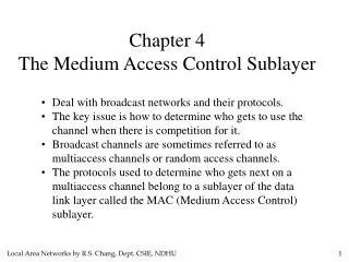
2. The Medium Access ControlSublayer • Network Classification • Use point-to-point connections - most WANs, except satellite. • Use broadcast channels - most LANs. • This chapter deals with broadcast networks and their protocol. • The objective is to allocate the channel to: • maximize channel utilization, and • minimize channel access delay.

3. Channel Allocation • Static Channel Allocation in LANs and MANs • Dynamic Channel Allocation in LANs and MANs

4. Static Channel Allocation • In static channel allocation, a subchannel is statically assigned to each station (computer or terminal). • For example, in FDM, a frequency band is assigned to each station. • This is inherently inefficient (w.r.t. channel utilization) for bursty traffic. • Note, however, the channel access delay is minimal.

5. Static Channel Allocation • We use the queueing system to analyze the above scheme. • Single station case: Let C = channel capacity (in bps) T = mean time delay to send one frame (in sec.) λ = arrival rate (in frames/sec.) 1/μ = mean frame size (in bits/frame) From queueing theory, we obtain: T = 1 / (μ C - λ) For example, if 1/ μ = 10,000 bits/frame, C = 100 Mbps, and λ = 5000 frames/sec, then T = 1 / ((1/104)(108) - 5000) = 1 / 5000 = 200 μsec. per frame.

6. Static Channel Allocation • N station case: Divide the channel up into N subchannels, each with capacity C/N. Let: λ /N = arrival rate at each station (divide the load). Then, TFDM = 1 / (μ(C/N) - λ/N) = N / (μC - λ) = N T. So, the N station case is N times worse than the 1 station case. For example, as above, N = 10 TFDM= 2 msec. per frame.

7. Dynamic Channel Allocation • Assumptions: • Station Model – N independent stations generate frames. • Single Channel – A single channel is available for all communication. • Collision – Frames that overlap in time destroy each other; this is called a COLLISION. All stations can detect collisions. The only errors are those caused by collisions.

8. Dynamic Channel Allocation • Assumptions: • Continuous Time means that transmission of frames can begin at any time. Slotted Time means that time is divided into discrete intervals, and frame transmission always begins at the start of a slot. • Carrier Sense means that stations can tell if the channel is in use by listening to the channel. No Carrier Sense means that stations cannot tell if the channel is in use by listening to the channel.

9. Pure ALOHA • In the Pure Aloha Protocol (by Abramson in 1970s), a station transmits the data whenever there is data to be sent. Then, the station listens to the channel to see if a collision occurred. If the frame was destroyed, the station waits for a random length of time and tries again. • Systems in which multiple users share a common channel in a way that can lead to conflicts are widely known as contention systems.

10. Pure ALOHA In pure ALOHA, frames are transmitted at completely arbitrary times.

11. Pure ALOHA - Analysis • Let FRAME TIME be the time required to transmit a standard, fixed-length frame; that is, (1/μC). • Assume there is an infinite population of stations that transmit frames according to a Poisson process with a mean of N frames transmitted per frame time. • Note, if N>1, the channel will not be able to handle the load. So, we expect 0<N<1. The offered load, G, is the total number of frames sent on the channel per frame time; that is, G = N + (number of retransmissions per frame time).

12. Pure ALOHA - Analysis • Let P0 = probability that no collisions occur during one frame time; that is, a transmission is successful. Then: the throughput, S = GP0 • Since the offered load is a Poisson distribution, with mean G, the probability that k frames are generated during a frame time is: Pr[k] = (Gk * e-G) / k! • So, Pr[0] = e-G. The probability of no other traffic during the vulnerable period is e-G e-G = e-2G. Thus, P0 = e-2G, and it follows that S = Ge-2G • dS/dG = e-2G (-2G + 1) = 0  G = 0.5 • Note, the maximum occurs when G = 0.5.S = 0.184.

13. FYI: Poisson Distribution • The Poisson Distributionis used to model the number of events occurring within a given time interval. • It is often used to model events such as the number of telephone calls at a business or the number of accidents at an intersection in a specific time period. • It is also useful in ecological studies, e.g., to model the number of prairie dogs found in a square mile of prairie. • The formula for the Poisson probability mass function is: p(x, λ) = e-λ λx / x! for x = 0, 1, 2, 3, …. λ is a is the shape parameter which indicates the average number of events in the given time interval.

14. FYI: Poisson Distribution • The following is the plot of the Poisson probability density function for four values of λ.

15. Pure ALOHA Vulnerable period for the shaded frame.

16. Slotted ALOHA • In slotted Aloha (by Roberts in 1972) A computer is not permitted to send whenever a carriage return is typed but wait for a time slot. • Time is divided into fixed slots of one frame time each. A station waits until the start of the next slot before transmitting a frame. Thus, P0 = e-G (the vulnerable period is only one time slot). S = G e-G Note that as G increases, the number of collisions increases exponentially. • Note, the maximum occurs when G = 1.S = 0.368. • Slotted Aloha can be used to allocate a shared cable channel.

17. Pure ALOHA Throughput versus offered traffic for ALOHA systems.

18. Carrier Sense Multiple Access (CSMA) • Protocols in which stations listen for a carrier (i.e. transmission) and act accordingly are called carrier sense protocols. • 1-persistent CSMA Channel Busy  Continue sensing until free and then grab. Channel Idle  Transmit with probability 1. Collision  Wait for a random length of time and try again. • nonpersistent CSMA: Channel Busy  Does not continually sense the channel. Wait for a random length of time and try again. Channel Idle  Transmit. Collision  Wait for a random length of time and try again.

19. Carrier Sense Multiple Access (CSMA) • p-persistent CSMA: Channel Busy  Continue sensing until free (same as idle). Channel Idle  Transmit with probability p, and defer transmitting until the next slot with probability q = 1-p. Collision  Wait for a random length of time and try again. • The nonpersistent CSMA has better channel utilization but longer delays than 1-persistent CSMA. • CSMA are an improvement over ALOHA because they ensure that no station begins to transmit when it senses the channel busy. • Another improvement is for stations to abort their transmissions as soon as they detect a collision. Quickly terminating damaged frames saves time and bandwidth. This protocol is called CSMA/CD (CSMA with Collision Detection).

20. Persistent and Nonpersistent CSMA Comparison of the channel utilization versus load for various random access protocols.

21. CSMA with Collision Detection CSMA/CD can be in one of three states: contention, transmission, or idle.

22. CSMA with Collision Detection • Stations detect collisions using analog hardware and abort transmissions immediately. • Let τ be the propagation delay (the time for a signal to propagate between the two farthest stations be τ). The contention interval is modeled as a slotted Aloha system with slot width 2τ. • Then, 2τ is the time required for a station to detect collision with certainty. For example, on a 1-km long coaxial cable, τ = 5 μsec. 2τ = 10 μsec to detect a collision.

23. Collision-Free Protocols • Assumptions: • There are N stations, uniquely numbered 0, 1, 2, …, N – 1. • Each contention period consists of N slots. • Data frames consist of d time units. • Basic Bit-Map Protocol • Low load  bit map is simply repeated over and over. • Low # stations: wait ~ 1.5N slots • High # stations: wait ~ 0.5N slots • The overhead to transmit a data frame is N bits. The channel efficiency at low load is d/(N + d) • The channel efficiency at high load dN /(N + dN) = d/(1 + d) • Binary Countdown – stations overwrite the low numbered stations, and low numbered stations give up.

24. Collision-Free Protocols The basic bit-map protocol.

25. Collision-Free Protocols The binary countdown protocol. A dash indicates silence.

26. Limited-Contention Protocols • Contention  Limited  Collision free (CSMA) contention (Binary Countdown) small delay for Good channel efficiency low load stations at high load • Analysis: Contention protocols (symmetric case) Let k = # of stations P = prob. that one station successfully requires the channel during a given slot. ρ = prob. that a station transmits a frame during a given slot.

27. Limited-Contention Protocols • Analysis: Contention protocols (Symmetric case) P = kρ(1 – ρ)k-1 ↓ prob. That the other stations do not transmit dP/dρ = –kρ(k – 1)(1 – ρ)k-2 + k(1 - ρ)k-1 = k(1 – ρ)k-2 [(ρ(k – 1) + (1 – ρ)] = k(1 – ρ)k-2 (-ρk + ρ + 1 – ρ) = 0  ρk = 1  ρ = 1/k P = k (1/k)(1 – 1/k)k-l = [(k – 1)/k]k-1 (4.4)

28. Limited-Contention Protocols Acquisition probability for a symmetric contention channel.

29. Limited-Contention Protocols • Idea: Limit the number of stations contending for a slot. • Question: How to assign stations to a slot? • Static assignment: One station/slot (group) Binary countdown Two stations/slot P = 1 – ρ2 ≈ 1 (ρ  0 collision is small) All stations/slot Slotted ALOHA

30. Adaptive Tree Walk Protocol • Use the algorithm devised by U.S. Army test for syphilis in 1943) • Example: There are 8 stations. Suppose that stations 0, 2, 4, and 5 want to transmit Slot 0 – All try Collision Slot 1 B Subtree try  Collision Slot 2 D Subtree try No collision – 0 Slot 3 E Subtree try No collision – 2 Slot 4 C Subtree try Collision Slot 5 F Subtree try Collision Slot 6 4 Slot 7 5 Slot 8  G Subtree try  No Collision

31. Adaptive Tree Walk Protocol The tree for eight stations.

32. Wavelength Division Multiple Access Protocols • Each station is assigned two channels: a narrow band control channel and a wide band data channel. • Each channel is divided into groups of time slots. All channels are synchronized by a single global clock. • The protocol support three traffic classes: • Constant data rate connection-oriented traffic such as uncompressed video. • Variable data rate connection-oriented traffic such as file transfer. • Datagram traffic such as UDP packet-oriented traffic.

33. Wavelength Division Multiple Access Protocols Wavelength division multiple access.

34. Wireless LAN Protocols • Because signal strength is not uniform throughout the space in which wireless LANs operate, carrier detection and collision may fail in the following ways: • Hidden nodes: • Hidden stations: Carrier sensing may fail to detect another station. For example, A and D. • Fading: The strength of radio signals diminished rapidly with the distance from the transmitter. For example, A and C. • Exposed nodes: • Exposed stations: B is sending to A. C can detect it. C might want to send to E but conclude it cannot transmit because C hears B. • Collision masking: The local signal might drown out the remote transmission. • The result scheme is carrier sensing multiple access with collision avoidance (CSMA/CA).

35. Wireless LAN configuration

36. Wireless LAN Protocols • Hidden station problem: A is transmitting to B. C cannot hear A. If C starts transmitting, it will interfere at B. • Exposed station problem: B is transmitting to A. C concludes that it may not send to D but the interference exists only between B and C. A wireless LAN. (a) A transmitting. (b) B transmitting.

37. MACA and MACAW • The sender transmits a RTS (Request To Send) frame. • The receiver replies with a CTS (Clear To Send) frame. • Neighbors • see CTS, then keep quiet. • see RTS but not CTS, then keep quiet until the CTS is back to the sender. • The receiver sends an ACK when receiving an frame. • Neighbors keep silent until see ACK. • Collisions • There is no collision detection. • The senders know collision when they don’t receive CTS. • They each wait for the exponential backoff time. • MACAW (MACA for Wireless) is a revision of MACA.

38. Wireless LAN Protocols The MACA protocol. (a) A sending an RTS to B. (b) B responding with a CTS to A.

39. Ethernet • Ethernet Cabling • Manchester Encoding • The Ethernet MAC Sublayer Protocol • The Binary Exponential Backoff Algorithm • Ethernet Performance • Switched Ethernet • Fast Ethernet • Gigabit Ethernet • IEEE 802.2: Logical Link Control • Retrospective on Ethernet

40. Ethernet Cabling • 10Base2 means that is operates at 10 Mbps, uses baseband signaling, and support segments up to 200 meters. • 10Base-T became dominant due to its use of existing wiring and the ease of maintenance . The most common kinds of Ethernet cabling.

41. Ethernet Cabling Three kinds of Ethernet cabling. (a) 10Base5, (b) 10Base2, (c) 10Base-T.

42. Ethernet Cabling • Different ways of wiring a building are shown as follows: Cable topologies. (a) Linear, (b) Spine, (c) Tree, (d) Segmented.

43. Ethernet Cabling • Devices used for connecting Ethernet cable: • A repeater is a physical layer device that receives, amplifies and retransmits the signal. • A hub will take a network packet and transmit it to all other ports on the hub. • A switch will take a network packet and transmit it only to a specific port on the switch that the packet is addressed to. So, a switch greatly reduces network transmissions thus providing better network throughput.

44. Ethernet Cabling • All Ethernet systems use Manchester encoding due to its simplicity (high at 0.85 V and low at -0.85 V). (a) Binary encoding, (b) Manchester encoding, (c) Differential Manchester encoding.

45. Ethernet MAC Sublayer Protocol • Preamble – used for sender and receiver to synchronize their clock. • Addresses • unique, 48-bit unicast address assigned to each adapter • example: 8:0:e4:b1:2 • broadcast: all 1s, the set of all recipient nodes • Multicast: first bit is 1,a group of recipient nodes Frame formats. (a) DIX Ethernet, (b) IEEE 802.3.

46. Ethernet Transmit Algorithm • If line is idle: • send immediately • upper bound message size of 1500 bytes • must wait some time (9.6µs) between back-to-back frames • If line is busy: • wait until idle and transmit immediately • called 1-persistent(a frame to send transmits with probability 1)

47. The Binary Exponential Backoff Algorithm • If collision • Time is divided into discrete slots whose length is equal to the worst-case round-trip propagation time on the ether (2τ). • minimum frame is 64 bytes (header + 46 bytes of data) = 512 bits • Channel capacity 10 Mbps, 512/10 M = 51.2µ • delay and try again (binary exponential backoff) • 1st time: waits 0 or 1 slotted time (51.2µs) • 2nd time: waits 0, 1, 2, or 3 slotted time • nth time: kslotted time, for randomly selected k=0..2n - 1 • Frozen at 1023 slots and give up after several tries (usually 16)

48. Ethernet MAC Sublayer Protocol

49. Ethernet Performance Efficiency of Ethernet at 10 Mbps with 512-bit slot times.

50. Switched Ethernet • To deal with increased load, the switched Ethernet is devised with a switch to route the frame to the destination. A simple example of switched Ethernet.