Data Warehousing & OLAP

1. Data Warehousing & OLAP Yannis Kotidis AT&T Labs-Research

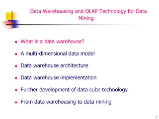
2. What is Data Warehouse? • “A data warehouse is a subject-oriented, integrated, time-variant, and nonvolatile collection of data in support of management’s decision-making process.”—W. H. Inmon • A Data Warehouse is used for On-Line-Analytical-Processing: “Class of tools that enables the user to gain insight into data through interactive access to a wide variety of possible views of the information” • 3 Billion market worldwide [1999 figure, olapreport.com] • Retail industries: user profiling, inventory management • Financial services: credit card analysis, fraud detection • Telecommunications: call analysis, fraud detection

3. Data Warehouse Initiatives • Organized around major subjects, such as customer, product, sales • integrate multiple, heterogeneous data sources • exclude data that are not useful in the decision support process • Focusing on the modeling and analysis of data for decision makers, not on daily operations or transaction processing • emphasis is on complex, exploratory analysis not day-to-day operations • Large time horizon for trend analysis (current and past data) • Non-Volatile store • physically separate store from the operational environment

4. Data Warehouse Architecture • Extract data from operational data sources • clean, transform • Bulk load/refresh • warehouse is offline • OLAP-server provides multidimensional view • Multidimensional-olap (Essbase, oracle express) • Relational-olap (Redbrick, Informix, Sybase, SQL server)

5. Why do we need all that? • Operational databases are for On Line Transaction Processing • automate day-to-day operations (purchasing, banking etc) • transactions access (and modify!) a few records at a time • database design is application oriented • metric: transactions/sec • Data Warehouse is for On Line Analytical Processing (OLAP) • complex queries that access millions of records • need historical data for trend analysis • long scans would interfere with normal operations • synchronizing data-intensive queries among physically separated databases would be a nightmare! • metric: query response time

6. Examples of OLAP • Comparisons (this period v.s. last period) • Show me the sales per region for this year and compare it to that of the previous year to identify discrepancies • Multidimensional ratios (percent to total) • Show me the contribution to weekly profit made by all items sold in the northeast stores between may 1 and may 7 • Ranking and statistical profiles (top N/bottom N) • Show me sales, profit and average call volume per day for my 10 most profitable salespeople • Custom consolidation (market segments, ad hoc groups) • Show me an abbreviated income statement by quarter for the last four quarters for my northeast region operations

7. Store 800 Product Multidimensional Modeling • Example: compute total sales volume per product and store

8. PRODUCT LOCATION TIME category region year product country quarter statemonth week city day store Dimensions and Hierarchies • A cell in the cube may store values (measurements) relative to the combination of the labeled dimensions DIMENSIONS city Sales of DVDs in NY in August NY DVD product month August

9. PRODUCT LOCATION TIME category region year product country quarter statemonth week city day store Common OLAP Operations • Roll-up: move up the hierarchy • e.g given total sales per city, we can roll-up to get sales per state • Drill-down: move down the hierarchy • more fine-grained aggregation • lowest level can be the detail records (drill-through)

10. Pivoting • Pivoting: aggregate on selected dimensions • usually 2 dims (cross-tabulation)

11. Slice and Dice Queries • Slice and Dice: select and project on one or more dimensions customers product store customer = “Smith”

12. Roadmap • What is a data warehouse and what it is for • What are the differences between OLTP and OLAP • Multi-dimensional data modeling • Data warehouse design • the star schema, bitmap indexes • The Data Cube operator • semantics and computation • Aggregate View Selection • Dynamic View Management • Other Issues

13. Data Warehouse Design • Most data warehouses adopt a star schema to represent the multidimensional model • Each dimension is represented by a dimension-table • LOCATION(location_key,store,street_address,city,state,country,region) • dimension tables are not normalized • Transactions are described through a fact-table • each tuple consists of a pointer to each of the dimension-tables (foreign-key) and a list of measures (e.g. sales $$$)

14. Star Schema Example TIME PRODUCT time_key day day_of_the_week month quarter year product_key product_name category brand color supplier_name SALES time_key product_key location_key units_sold amount LOCATION { location_key store street_address city state country region measures

15. Advantages of Star Schema • Facts and dimensions are clearly depicted • dimension tables are relatively static, data is loaded (append mostly) into fact table(s) • easy to comprehend (and write queries) • “Find total sales per product-category in our stores in Europe” • SELECT PRODUCT.category, SUM(SALES.amount) • FROM SALES, PRODUCT,LOCATION • WHERE SALES.product_key = PRODUCT.product_key • AND SALES.location_key = LOCATION.location_key • AND LOCATION.region=“Europe” • GROUP BY PRODUCT.category

16. Star Schema Query Processing TIME PRODUCT time_key day day_of_the_week month quarter year product_key product_name category brand color supplier_name SALES Pcategory time_key product_key location_key units_sold amount JOIN JOIN LOCATION { location_key store street_address city state country region measures Sregion=“Europe”

17. Indexing OLAP Data: Bitmap Index • Each value in the column has a bit vector: • The i-th bit is set if the i-th row of the base table has the value for the indexed column • The length of the bit vector: # of records in the base table • Mainly intended for small cardinality domains LOCATION Index on Region

18. 1 1 1 1 Join-Index • Join index relates the values of the dimensions of a star schema to rows in the fact table. • a join index on region maintains for each distinct region a list of ROW-IDs of the tuples recording the sales in the region • Join indices can span multiple dimensions OR • can be implemented as bitmap-indexes (per dimension) • use bit-op for multiple-joins SALES LOCATION R102 R117 R118 R124 region = Africa region = America region = Asia region = Europe

19. Problem Solved? • “Find total sales per product-category in our stores in Europe” • Join-index will prune ¾ of the data (uniform sales), but the remaining ¼ is still large (several millions transactions) • Index is unclustered • High level aggregations are expensive!!!!! • long scans to get the data • hashing or sorting necessary for group-bys LOCATON region country state city store Long Query Response Times Pre-computation is necessary

20. Multiple Simultaneous Aggregates 4 Group-bys here: (store,product) (store) (product) () Cross-Tabulation (products/store) Need to write 4 queries!!! Sub-totals per store Total sales Sub-totals per product

21. The Data Cube Operator (Gray et al) • All previous aggregates in a single query: SELECT LOCATION.store, SALES.product_key, SUM (amount) FROM SALES, LOCATION WHERE SALES.location_key=LOCATION.location_key CUBE BY SALES.product_key, LOCATION.store Challenge: Optimize Aggregate Computation

22. Relational View of Data Cube Store Product_key sum(amout) 1 1 454 1 4 925 2 1 468 2 2 800 3 1 296 3 3 240 4 1 625 4 3 240 4 4 745 1 ALL 1379 1 ALL 1268 1 ALL 536 1 ALL 1937 ALL 1 1870 ALL 2 800 ALL 3 780 ALL 4 1670 ALL ALL 5120 SELECT LOCATION.store, SALES.product_key, SUM (amount) FROM SALES, LOCATION WHERE SALES.location_key=LOCATION.location_key CUBE BY SALES.product_key, LOCATION.store

23. Quarter 2Qtr 1Qtr sum 3Qtr 4Qtr DVD Product America PC VCR sum Europe Region Asia sum All, All, All Data Cube: Multidimensional View Total annual sales of DVDs in America

24. Other Extensions to SQL • Complex aggregation at multiple granularities (Ross et. all 1998) • Compute multiple dependent aggregates • Other proposals: the MD-join operator (Chatziantoniou et. all 1999] SELECT LOCATION.store, SALES.product_key, SUM (amount) FROM SALES, LOCATION WHERE SALES.location_key=LOCATION.location_key CUBE BY SALES.product_key, LOCATION.store: R SUCH THAT R.amount = max(amount)

25. product,store,quarter product,quarter store,quarter product, store quarter product store none Data Cube Computation • Model dependencies among the aggregates: most detailed “view” can be computed from view (product,store,quarter) by summing-up all quarterly sales

26. product,store,quarter product,quarter store,quarter product, store quarter product store none Computation Directives • Hash/sort based methods (Agrawal et. al. VLDB’96) • Smallest-parent • Cache-results • Amortize-scans • Share-sorts • Share-partitions

27. B Alternative Array-based Approach • Model data as a sparse multidimensional array • partition array into chunks (a small sub-cube which fits in memory). • fast addressing based on (chunk_id, offset) • Compute aggregates in “multi-way” by visiting cube cells in the order which minimizes the # of times to visit each cell, and reduces memory access and storage cost. What is the best traversing order to do multi-way aggregation?

28. Reality check:too many views! • 2n views for n dimensions (no-hierarchies) • Storage/update-time explosion • More pre-computation doesn’t mean better performance!!!!

29. product,store,quarter product,quarter store,quarter product, store quarter product store none How to choose among the views? • Use some notion of benefit per view • Limit: disk space or maintenance-time Hanarayan et al SIGMOD’96: Pick views greedily until space is filled Catch: quadratic in the number of views, which is exponential!!!

30. View Selection Problem • Selection is based on a workload estimate (e.g. logs) and a given constraint (disk space or update window) • NP-hard, optimal selection can not be computed > 4-5 dimensions • greedy algorithms (e.g. [Harinarayan96]) run at least in polynomial time in the number of views i.e exponential in the number of dimensions!!! • Optimal selection can not be approximated [Karloff99] • greedy view selection can behave arbitrary bad • Lack of good models for a cost-based optimization!

31. Problem Generalization • View Management Problem: Materialize and maintain the right subset of views with respect to the workload and the available resources • What is the workload? • “Farmers” v.s. “Explorers” [Inmon99] • Pre-compiled queries (report generating tools, data mining) • Ad-hoc analysis (unpredictable) • What are the resources? • Disk space (getting cheaper) • Update window (getting smaller)

32. DynaMat: A Dynamic View Management System • Continuous management based on disk space and update window restrictions • Engage views whenever possible for incoming queries • e.g. infer monthly sales out of pre-computed daily sales • support both ad-hoc and pre-compiled queries • Exploit dependencies among the views to maintain the best subset of them within the given update window

33. System Overview • Utilize a dedicated disk space (View Pool) for results of past queries • Engage stored results for answering new queries • Amortize query execution cost through multiple uses of the result DW base tables Query Interface Aggregate Locator Admission Control User View Pool

34. Space bound Time bound The Space & Time Bounds • Pool utilization increases between updates • Space bound: new results compete with stored aggregates for the limited space • Time bound: results are evicted from the pool due to the update-time window

35. product f1 f2 link store customer goodness(f) = accesses(f) / (t-tlast_access) * cost(f) / size(f) size in pages staleness re-computation cost number of accesses Dynamic View Management • Space and time restrictions will lead us to evict materialized aggregates • Not a traditional caching problem • aggregates don’t have the same size,cost, cost/size • aggregates are not independent • costs are dynamic

36. Deltas Incremental product Re-compute updated results store customer Exploiting Dependencies For Updates • For each stored aggregate compute minimum update cost UC(f) • incrementally from deltas • re-computation from father • shared maintenance cost • Total Update Cost: f

37. Roadmap • What is a data warehouse and what it is for • What are the differences between OLTP and OLAP • Multi-dimensional data modeling • Data warehouse design • the star schema, bitmap indexes • The Data Cube operator • semantics and computation • Aggregate View Selection • Dynamic View Management • Other Issues

38. Other Issues • Fact+Dimension tables in the DW are views of tables stored in the sources • Lots of view maintenance problems • correctly reflect asynchronous changes at the sources • making views self-maintainable • Interactive queries (on-line aggregation) • e.g. show running-estimates + confidence intervals • Computing Iceberg queries efficiently • Approximation • rough-estimates for hi-level aggregates are often good-enough • histogram, wavelet, sampling based techniques (e.g. AQUA)

39. The End • Thank you!