Download
1 / 59
590 likes | 637 Views
Understand the principles behind network layer services: IP routing including path selection, router functionality, and implementation in the Internet. Explore routing algorithms, call setup, and network architecture.

E N D
References • Text books: • Computer Networking: A Top-Down Approach Featuring the Internet, 2/e by Kurose and Ross
Chapter goals: understand principles behind network layer services: routing (path selection) dealing with scale how a router works instantiation and implementation in the Internet Overview: network layer services IP (Internet Protocol) routing principles: path selection Lecture 5: Network Layer
Outline 4.1 Introduction and Network Service Models 4.2 The Internet (IP) Protocol 4.3 Routing Principles
deliver packets from sending to receiving hosts network layer protocols in every host, router three important functions: path determination: route taken by packets from source to dest. Routing algorithms forwarding: move packets from router’s input to appropriate router output call setup:some network architectures require router call setup along path before data flows network data link physical network data link physical network data link physical network data link physical network data link physical network data link physical network data link physical network data link physical application transport network data link physical application transport network data link physical Network layer functions
Key Network-Layer Functions • forwarding: move packets from router’s input to appropriate router output • routing: determine route taken by packets from source to dest. • Routing algorithms analogy: • routing: process of planning trip from source to dest • forwarding: process of getting through single interchange
Interplay between routing and forwarding routing algorithm local forwarding table header value output link 0100 0101 0111 1001 3 2 2 1 value in arriving packet’s header 1 0111 2 3
Q: What service model for “channel” transporting packets from sender to receiver? guaranteed bandwidth? preservation of inter-packet timing (no jitter)? loss-free delivery? in-order delivery? congestion feedback to sender? Network service model The most important abstraction provided by network layer: ? ? virtual circuit or datagram? ? service abstraction The complexity of the network layer depends on the service model it provides:
Network Layer Service Models Guarantees ? Network Architecture Internet ATM ATM ATM ATM Service Model best effort CBR VBR ABR UBR Congestion feedback no (inferred via loss) no congestion no congestion yes no Bandwidth none constant rate guaranteed rate guaranteed minimum none Loss no yes yes no no Order no yes yes yes yes Timing no yes yes no no • Internet model being extended: IntServ, DiffServ • multimedia networking ATM: Asynchronous Transfer Mode; CBR: Constant Bit Rate; V: Variable; A: available; U: User
“source-to-dest path behaves much like telephone circuit” performance-wise network actions along source-to-dest path application transport network data link physical application transport network data link physical Virtual circuits 6. Receive data 5. Data flow begins 4. Call connected 3. Accept call 1. Initiate call 2. incoming call
call setup, teardown for each call before data can flow each packet carries VC identifier (not destination host ID) every router on source-dest path maintains “state” for each passing connection transport-layer connection only involved two end systems link, router resources (bandwidth, buffers) may be allocated to VC to get circuit-like perf. Virtual circuits • used to setup, maintain teardown VC • used in ATM, frame-relay, X.25 • not used in today’s Internet
no call setup at network layer routers: no state about end-to-end connections no network-level concept of “connection” Forwarded: using destination host address packets between same source-dest pair may take different paths application transport network data link physical application transport network data link physical Datagram networks: Internet’s model 1. Send data 2. Receive data
Internet (Datagram) data exchange among computers “elastic” service, no strict timing req. “smart” end systems (computers) can adapt, perform control, error recovery simple inside network, complexity at “edge” heterogeneous link types different characteristics uniform service difficult Asynchronous Transfer Mode - ATM (VC) evolved from telephony human conversation: strict timing, reliability requirements need for guaranteed service “dumb” end systems telephones complexity inside network Datagram or VC network: why?
Outline 4.1 Introduction and Network Service Models 4.2 The Internet (IP) Protocol • IPv4 addressing • Moving a datagram from source to destination • Datagram format • IP fragmentation 4.3 Routing Principles
Host, router network layer functions: • ICMP protocol • error reporting • router “signaling” • IP protocol • addressing conventions • datagram format • packet handling conventions • Routing protocols • path selection • RIP, OSPF, BGP forwarding table The Internet Network layer Transport layer: TCP, UDP Network layer Link layer physical layer
IP address: 32-bit identifier for host, router interface interface: connection between host/router and physical link router’s typically have multiple interfaces host may have multiple interfaces IP addresses associated with each interface 223.1.1.2 223.1.2.1 223.1.3.27 223.1.3.1 223.1.3.2 223.1.2.2 IP Addressing: introduction 223.1.1.1 223.1.2.9 223.1.1.4 223.1.1.3 223.1.1.1 = 11011111 00000001 00000001 00000001 223 1 1 1
IP address: network part (high order bits) host part (low order bits) What’s a network ? (from IP address perspective) device interfaces with same network part of IP address can physically reach each other without intervening router IP Addressing 223.1.1.1 223.1.2.1 223.1.1.2 223.1.2.9 223.1.1.4 223.1.2.2 223.1.1.3 223.1.3.27 LAN 223.1.3.2 223.1.3.1 network consisting of 3 IP networks (for IP addresses starting with 223, first 24 bits are network address)
multicast address 1110 network host 110 network 10 host IP Addresses given notion of “network”, let’s re-examine IP addresses: “classful” addressing: class 1.0.0.0 to 127.255.255.255 A network 0 host 128.0.0.0 to 191.255.255.255 B 192.0.0.0 to 223.255.255.255 C 224.0.0.0 to 239.255.255.255 D 32 bits
host part network part 11001000 0001011100010000 00000000 200.23.16.0/23 IP addressing: CIDR • Classful addressing: • inefficient use of address space, address space exhaustion • e.g., class B net allocated enough addresses for 65K hosts, even if only 2K hosts in that network • CIDR:Classless InterDomain Routing (“cider”) • network portion of address of arbitrary length • address format (1): a.b.c.d/x, where x is # bits in network portion of address
host part host part network part network part 11001000 0001011100010000 00000000 1111111111111111 11111110 00000000 200.23.16.0/23 255.255.254.0 IP addressing: CIDR • CIDR:Classless InterDomain Routing • network portion of address of arbitrary length • address format (2): address + mask IP address IP mask
Network partitioning • You are given a pool of 220.23.16.0/24 IP addresses to assign to hosts and routers in the system (right): • How many separate networks are there in the system? • Partition the given address space and assign addresses to the networks.
Network partitioning • You are given a pool of 220.23.16.0/24 IP addresses to assign to hosts and routers in the system (right): • How many separate networks are there in the system? 6 • Partition the given address space and assign addresses to the networks.
IP datagram: A E B source IP addr misc fields dest IP addr data 223.1.1.1 223.1.2.1 223.1.1.2 223.1.2.9 223.1.1.4 223.1.2.2 223.1.1.3 223.1.3.27 Dest. Net. next router Nhops 223.1.1 1 223.1.3.2 223.1.3.1 223.1.2 223.1.1.4 2 223.1.3 223.1.1.4 2 Getting a datagram from source to dest. forwarding table in A • datagram remains unchanged, as it travels source to destination • addr fields of interest here
B E A 223.1.1.1 223.1.2.1 223.1.1.2 223.1.2.9 223.1.1.4 223.1.2.2 223.1.1.3 223.1.3.27 Dest. Net. next router Nhops 223.1.1 1 223.1.3.2 223.1.3.1 223.1.2 223.1.1.4 2 223.1.3 223.1.1.4 2 Getting a datagram from source to dest. forwarding table in A misc fields data 223.1.1.1 223.1.1.3 Starting at A, send IP datagram addressed to B: • look up net. address of B in forwarding table • find B is on same net. as A • link layer will send datagram directly to B inside link-layer frame • B and A are directly connected
E A B 223.1.1.1 223.1.2.1 223.1.1.2 223.1.2.9 223.1.1.4 223.1.2.2 223.1.1.3 223.1.3.27 Dest. Net. next router Nhops 223.1.1 1 223.1.3.2 223.1.3.1 223.1.2 223.1.1.4 2 223.1.3 223.1.1.4 2 Getting a datagram from source to dest. forwarding table in A misc fields data 223.1.1.1 223.1.2.2 Starting at A, dest. E: • look up network address of E in forwarding table • E on different network • A, E not directly attached • routing table: next hop router to E is 223.1.1.4 • link layer sends datagram to router 223.1.1.4 inside link-layer frame • datagram arrives at 223.1.1.4 • continued…..
Dest. Net router Nhops interface B A E 223.1.1 - 1 223.1.1.4 223.1.2 - 1 223.1.2.9 223.1.3 - 1 223.1.3.27 223.1.1.1 223.1.2.1 223.1.1.2 223.1.2.9 223.1.1.4 223.1.2.2 223.1.1.3 223.1.3.27 223.1.3.2 223.1.3.1 Getting a datagram from source to dest. forwarding table in router misc fields data 223.1.1.1 223.1.2.2 Arriving at 223.1.1.4, destined for 223.1.2.2 • look up network address of E in router’s forwarding table • E on same network as router’s interface 223.1.2.9 • router, E directly attached • link layer sends datagram to 223.1.2.2 inside link-layer frame via interface 223.1.2.9 • datagram arrives at 223.1.2.2!!! (hooray!)
IP addresses: how to get one – host ? Q: How does host get IP address? • hard-coded by system admin in a file • Wintel: control-panel->network->configuration->tcp/ip->properties • UNIX: /etc/rc.config • DHCP:Dynamic Host Configuration Protocol: dynamically get address from as server • “plug-and-play”
DHCP: Dynamic Host Configuration Protocol Goal: allow host to dynamically obtain its IP address from network server when it joins network • Allows reuse of addresses (only hold address while connected an “on” • Support for mobile users who want to join network
A B E DHCP client-server scenario 223.1.2.1 DHCP 223.1.1.1 server 223.1.1.2 223.1.2.9 223.1.1.4 223.1.2.2 arriving DHCP client needs address in this network 223.1.1.3 223.1.3.27 223.1.3.2 223.1.3.1 • host broadcasts “DHCP discover” msg • DHCP server responds with “DHCP offer” msg • host requests IP address: “DHCP request” msg • DHCP server sends address: “DHCP ack” msg
IP protocol version number 32 bits total datagram length (bytes) header length (bytes) type of service head. len ver length for fragmentation/ reassembly fragment offset “type” of data flgs 16-bit identifier max number remaining hops (decremented at each router) upper layer time to live Internet checksum 32 bit source IP address 32 bit destination IP address upper layer protocol to deliver payload to E.g. timestamp, record route taken, specify list of routers to visit. Options (if any) data (variable length, typically a TCP or UDP segment) IP datagram format how much overhead with TCP? • 20 bytes of TCP • 20 bytes of IP • = 40 bytes + app layer overhead
network links have MTU (max.transfer size) - largest possible link-level frame. different link types, different MTUs large IP datagram divided (“fragmented”) within net one datagram becomes several datagrams “reassembled” only at final destination IP header bits used to identify, order related fragments IP Fragmentation & Reassembly fragmentation: in: one large datagram out: 3 smaller datagrams reassembly
length =1500 length =1500 length =4000 length =1040 ID =x ID =x ID =x ID =x fragflag =0 fragflag =1 fragflag =0 fragflag =1 offset =0 offset =0 offset =1480 offset =2960 One large datagram becomes several smaller datagrams IP Fragmentation and Reassembly Example • 4000 byte datagram • MTU = 1500 bytes
Outline 4.1 Introduction and Network Service Models 4.2 The Internet (IP) Protocol 4.3 Routing Principles • Link state routing • Distance vector routing
Graph abstraction for routing algorithms: graph nodes are routers graph edges are physical links link cost: delay, $ cost, or congestion level A D E B F C Routing protocol Routing 5 Goal: determine a “good” path (sequence of routers) thru network from source to dest. 3 5 2 2 1 3 1 2 1 • “good” path: • typically means minimum cost path • other def’s possible
Global or decentralized information? Global: all routers have complete topology, link cost info “link state” algorithms Decentralized: router knows physically-connected neighbors, link costs to neighbors iterative process of computation, exchange of info with neighbors “distance vector” algorithms Static or dynamic? Static: routes change slowly over time Dynamic: routes change more quickly periodic update in response to link cost changes Routing Algorithm classification
Dijkstra’s algorithm net topology, link costs known to all nodes accomplished via “link state broadcast” all nodes have same info computes least cost paths from one node (‘source”) to all other nodes gives routing table for that node Notation: c(i,j): link cost from node i to j. cost infinite if not direct neighbors D(v): current value of cost of path from source to dest V p(v): predecessor node along path from source to v, that is next v N: set of nodes whose least cost path definitively known A Link-State Routing Algorithm
Dijsktra’s Algorithm 1 Initialization: 2 N = {A} 3 for all nodes v 4 if v adjacent to A 5 then D(v) = c(A,v) 6 else D(v) = infinity 7 8 Loop 9 find w not in N such that D(w) is a minimum 10 add w to N 11 update D(v) for all v adjacent to w and not in N: 12 D(v) = min( D(v), D(w) + c(w,v) ) 13 /* new cost to v is either old cost to v or known 14 shortest path cost to w plus cost from w to v */ 15 until all nodes in N
A D B E F C Dijkstra’s algorithm: example D(B),p(B) 2,A 2,A 2,A D(D),p(D) 1,A D(C),p(C) 5,A 4,D 3,E 3,E D(E),p(E) infinity 2,D Step 0 1 2 3 4 5 start N A AD ADE ADEB ADEBC ADEBCF D(F),p(F) infinity infinity 4,E 4,E 4,E 5 3 5 2 2 1 3 1 2 1
Use Dijkstra’s shortest path algorithm to compute the shortest path from A to all network nodes.
Algorithm complexity: n nodes each iteration: need to check all nodes, w, not in N n*(n+1)/2 comparisons: O(n**2) more efficient implementations possible: O(nlogn) Dijkstra’s algorithm, discussion
iterative: continues until no nodes exchange info. self-terminating: no “signal” to stop asynchronous: nodes need not exchange info/iterate in lock step! distributed: each node communicates only with directly-attached neighbors Key Idea Given my distance to a neighboring node Given the distances from the neighboring nodes to remote nodes My distances to remote nodes Distance Vector Routing Algorithm
Distance Table data structure each node has its own row for each possible destination column for each directly-attached neighbor to node example: in node X, for dest. Y via neighbor Z: distance from X to Y, via Z as next hop X = D (Y,Z) Z c(X,Z) + min {D (Y,w)} = w Distance Vector Routing Algorithm via X D () Y Z Y 1 7 Z 2 5 destination
cost to destination via E D () A B C D A 1 7 6 4 B 14 8 9 11 D 5 5 4 2 destination A D B E C E E E D (C,D) D (A,D) D (A,B) D B D c(E,D) + min {D (C,w)} c(E,D) + min {D (A,w)} c(E,B) + min {D (A,w)} = = = w w w = = = 8+6 = 14 2+2 = 4 2+3 = 5 Distance Table: example 1 7 2 8 ? ? 1 2 loop! loop!
cost to destination via E D () A B C D A 1 7 6 4 B 14 8 9 11 D 5 5 4 2 destination Distance table gives routing table Outgoing link to use, cost A B C D A,1 D,5 D,4 D,2 destination Routing table Distance table
Iterative, asynchronous: each local iteration caused by: message from neighbor: its least cost path change from neighbor Distributed: each node notifies neighbors only when its least cost path to any destination changes neighbors then notify their neighbors if necessary Distance Vector Routing: overview Each node: wait for (msg from neighbor) recompute distance table if least cost path to any dest has changed, notify neighbors
Distance Vector Algorithm: At all nodes, X: 1 Initialization: 2 for all adjacent nodes v: 3 D (*,v) = infinity /* the * operator means "for all rows" */ 4 D (v,v) = c(X,v) /* direct neighbors */ 5 for all destinations, y 6 send min D (y,w) to each neighbor /* w over all X's neighbors */ X X X w
Distance Vector Algorithm (cont.): 8 loop 9 wait (until I receive update from neighbor V) 10 11if (update received from V wrt destination Y) 12/* shortest path from V to some Y has changed */ 13 /* V has sent a new value for its min DV(Y,w) */ 14 /* call this received new value is "newval" */ 15 for the single destination y: D (Y,V) = c(X,V) + newval 16 17if we have a new min D (Y,w) for any destination Y 18 send new value of min D (Y,w) to all neighbors 19 20forever w X X w X w
2 1 7 Y Z X X c(X,Y) + min {D (Z,w)} c(X,Z) + min {D (Y,w)} D (Y,Z) D (Z,Y) = = w w = = 7+1 = 8 2+1 = 3 X Z Y Distance Vector Algorithm: example
2 1 7 X Z Y Distance Vector Algorithm: example ?
2 1 7 X Z Y Distance Vector Algorithm: example 2 4 1 5