Download
1 / 45
450 likes | 685 Views
CompSci 356: Computer Network Architectures Lecture 22: Overlay Networks. Xiaowei Yang xwy@cs.duke.edu. Overview. Overlay networks Unstructured Structured Distributed Hash Tables. What is an overlay network?. A logical network implemented on top of a lower-layer network

E N D
CompSci 356: Computer Network Architectures Lecture 22: Overlay Networks Xiaowei Yang xwy@cs.duke.edu
Overview • Overlay networks • Unstructured • Structured • Distributed Hash Tables
What is an overlay network? • A logical network implemented on top of a lower-layer network • Can recursively build overlay networks • An overlay link is defined by the application
Ex: Virtual Private Networks • Links are defined as IP tunnels • May include multiple underlying routers
Unstructured Overlay Networks • Overlay links form random graphs • No defined structure • Examples • Gnutella: links are peer relationships • One node that runs Gnutella knows some other Gnutella nodes • BitTorrent • A node and nodes in its view
Structured Networks • A node forms links with specific neighbors to maintain a certain structure of the network • Pros • More efficient data lookup • More reliable • Cons • Difficult to maintain the graph structure • Examples • End-system multicast: overlay nodes form a multicast tree • Distributed Hash Tables
DHT Overview • Used in the real world • BitTorrent tracker implementation • Content distribution networks • What problems do DHTs solve? • How are DHTs implemented?
Background • A hash table is a data structure that stores (key, object) pairs. • Key is mapped to a table index via a hash function for fast lookup. • Content distribution networks • Given an URL, returns the object
Example of a Hash table: a web cache • Client requests http://www.cnn.com • Web cache returns the page content located at the 1st entry of the table. 0 1 2
DHT: why? • If the number of objects is large, it is impossible for any single node to store it. • Solution: distributed hash tables. • Split one large hash table into smaller tables and distribute them to multiple nodes
K K K V V V DHT V K
A content distribution network • A single provider that manages multiple replicas • A client obtains content from a close replica
Basic function of DHT • DHT is a “virtual” hash table • Input: a key • Output: a data item • Data Items are stored by a network of nodes. • DHT abstraction • Input: a key • Output: the node that stores the key • Applications handle key and data item association.
K K K K K V V V V V DHT: a visual example (K1, V1) Insert (K1, V1)
K K K K K V V V V V DHT: a visual example (K1, V1) Retrieve K1
Desired goals of DHT • Scalability: each node does not keep much state • Performance: small look up latency • Load balancing: no node is overloaded with a large amount of state • Dynamic reconfiguration: when nodes join and leave, the amount of state moved from nodes to nodes is small. • Distributed: no node is more important than others.
A straw man design • Suppose all keys are integers • The number of nodes in the network is n • id = key % n (0, V1) (3, V2) 0 (1, V3) (4, V4) (2, V5) (5, V6) 1 2
When node 2 dies • A large number of data items need to be rehashed. (0, V1) 0 (2, V5) (4, V4) (1, V3) (3, V2) 1 (5, V6)
Fix: consistent hashing • A node is responsible for a range of keys • When a node joins or leaves, the expected fraction of objects that must be moved is the minimum needed to maintain a balanced load. • All DHTs implement consistent hashing
Basic components of DHTs • Overlapping key and node identifier space • Hash(www.cnn.com/image.jpg) a n-bit binary string • Nodes that store the objects also have n-bit string as their identifiers • Building routing tables • Next hops (structure of a DHT) • Distance functions • These two determine the geometry of DHTs • Ring, Tree, Hybercubes, hybrid (tree + ring) etc. • Handle node join and leave • Lookup and store interface
Chord: basic idea • Hash both node id and key into a m-bit one-dimension circular identifier space • Consistent hashing: a key is stored at a node whose identifier is closest to the key in the identifier space • Key refers to both the key and its hash value.
Chord: ring topology Key 5 K5 Node 105 N105 K20 Circular 7-bit ID space N32 N90 K80 A key is stored at its successor: node with next higher ID
Chord: how to find a node that stores a key? • Solution 1: every node keeps a routing table to all other nodes • Given a key, a node knows which node id is successor of the key • The node sends the query to the successor • What are the advantages and disadvantages of this solution?
Solution 2: every node keeps a routing entry to the node’s successor (a linked list) N120 N10 “Where is key 80?” N105 N32 “N90 has K80” N90 K80 N60
Simple lookup algorithm Lookup(my-id, key-id) n = my successor if my-id < n < key-id call Lookup(key-id) on node n // next hop else return my successor // done • Correctness depends only on successors • Q1: will this algorithm miss the real successor? • Q2: what’s the average # of lookup hops?
Solution 3: “Finger table” allows log(N)-time lookups • Analogy: binary search ½ ¼ 1/8 1/16 1/32 1/64 1/128 N80
Finger i points to successor of n+2i-1 N120 112 ½ • The ith entry in the table at node n contains the identity of the first node s that succeeds n by at least 2i-1 • A finger table entry includes Chord Id and IP address • Each node stores a small table log(N) ¼ 1/8 1/16 1/32 1/64 1/128 N80
0 7 1 6 2 5 3 4 Chord finger table example 0+20 1 Keys: 5,6 0+21 3 0 0+22 2 3 Keys: 1 3 3 0 5 4 0 Keys: 2 5 0 0 7
Lookup with fingers Lookup(my-id, key-id) look in local finger table for highest node n s.t. my-id < n < key-id if n exists call Lookup(key-id) on node n // next hop else return my successor // done
1 1 Keys: 5,6 2 3 0 0 4 7 1 6 2 5 3 4 Chord lookup example • Lookup(1,6) • Lookup(1,2) 2 3 Keys: 1 3 3 0 5 4 0 Keys: 2 5 0 0 7
Node join • Maintain the invariant • Each node’ successor is correctly maintained • For every node k, node successor(k) answers for key k. It’s desirable that finger table entries are correct • Each nodes maintains a predecessor pointer • Tasks: • Initialize predecessor and fingers of new node • Update existing nodes’ state • Notify apps to transfer state to new node
Chord Joining: linked list insert • Node n queries a known node n’ to initialize its state • for its successor: lookup (n) N25 N36 1. Lookup(36) K30 K38 N40
Join (2) N25 2. N36 sets its own successor pointer N36 K30 K38 N40
Join (3) • Note that join does not make the network aware of n N25 3. Copy keys 26..36 from N40 to N36 N36 K30 K30 K38 N40
Join (4): stabilize N25 • Stabilize 1) obtains a node n’s successor’s predecessor x, and determines whether x should be n’s successor 2) notifies n’s successor n’s existence • N25 calls its successor N40 to return its predecessor • Set its successor to N36 • Notifies N36 it is predecessor • Update finger pointers in the background periodically • Find the successor of each entry i • Correct successors produce correct lookups 4. Set N25’s successor pointer N36 K30 N40 K38
Failures might cause incorrect lookup N120 N10 N113 N102 Lookup(90) N85 N80 N80 doesn’t know correct successor, so incorrect lookup
Solution: successor lists • Each node knows r immediate successors • After failure, will know first live successor • Correct successors guarantee correct lookups • Guarantee is with some probability • Higher layer software can be notified to duplicate keys at failed nodes to live successors
Choosing the successor list length • Assume 1/2 of nodes fail • P(successor list all dead) = (1/2)r • I.e. P(this node breaks the Chord ring) • Depends on independent failure • P(no broken nodes) = (1 – (1/2)r)N • r = 2log(N) makes prob. = 1 – 1/N
Lookup with fault tolerance Lookup(my-id, key-id) look in local finger table and successor-list for highest node n s.t. my-id < n < key-id if n exists call Lookup(key-id) on node n // next hop if call failed, remove n from finger table return Lookup(my-id, key-id) else return my successor // done
Chord performance • Per node storage • Ideally: K/N • Implementation: large variance due to unevenly node id distribution • Lookup latency • O(logN)
Comments on Chord • ID distance Network distance • Reducing lookup latency and locality • Strict successor selection • Can’t overshoot • Asymmetry • A node does not learn its routing table entries from queries it receives • Later work fixes these issues
Conclusion • Overlay networks • Structured vs Unstructured • Design of DHTs • Chord
Lab 3 Congestion Control • This lab is based on Lab 1, you don’t have to change much to make it work. • You are required to implement a congestion control algorithm • Fully utilize the bandwidth • Share the bottleneck fairly • Write a report to describe your algorithm design and performance analysis • You may want to implement at least • Slow start • Congestion avoidance • Fast retransmit and fast recovery • RTO estimator • New RENO is a plus. It handles multiple packets loss very well.
port: 10000 port: 20000 A1 on linux21 transmitting file1 A2 on linux22 receiving file1 port: 50002 port: 50001 bottleneck link L port: 50004 port: 50003 port: 30000 relayeron linux25 simulating the bottleneck port: 40000 B1 on linux23 transmitting file2 B2 on linux24 receiving file2 Lab 3 Congestion Control