Download
1 / 62
620 likes | 785 Views
Subwavelength Design: Lithography Effects and Challenges Part II: EDA Implications. Andrew B. Kahng, UCLA Computer Science Dept. ISQED-2000 Tutorial March 20, 2000. Forcing Trends in EDA. Silicon complexity and design complexity many opportunities to leave major $$$ on the table

E N D
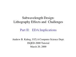
Subwavelength Design: Lithography Effects and Challenges Part II: EDA Implications Andrew B. Kahng, UCLA Computer Science Dept. ISQED-2000 Tutorial March 20, 2000
Forcing Trends in EDA • Silicon complexity and design complexity • many opportunities to leave major $$$ on the table • issues: physical effects of process, migratability • design rules more conservative, design waivers • device-level layout opts in cell-based methodologies • Verification cost increases dramatically • Prevention a necessary complement to checking • Successive approximation = design convergence • upstream activities pass intentions, assumptions downstream • downstream activities must be predictable • models of analysis/verification == objectives for synthesis
EDA Awareness of Process EDA wants to know as little as possible This part of tutorial: the unavoidable issues
Necessary Formulations, Flows • Upstream objectives want to capture downstream layout operations “transparently” • New problem formulations • PSM: more global phenomena, scalability issues • OPC: mostly local phenomena • function-driven corrections • hierarchical and reuse-centric regimes • New tool integrations
Features Conflict areas (<B) < B > B 0 180 0 Phase Assignment in PSM Assign 0, 180 phase regions such that: • (dark field) feature pairs with separation < B have opposite phases • (bright field) features with width < B are induced by adjacent phase regions with opposite phases (Dark field, neg resist) b b minimum separation or width, with phase shifting B minimum separation or width, without phase shifting
Conflict Graph Vertices: features (or phase regions) Edges: “conflicts” (necessary phase contrasts) (feature pairs with separation< B ) < B
Odd Cycles in Conflict Graph • Self-consistent phase assignment is not possible if there is an odd cycle in the conflict graph • Phase-assignable bipartite no odd cycles 0 phase 180 phase ??? phase
Breaking Odd Cycles • Must change the layout: • change feature dimensions, and/or • change spacings • PSM phase-assignability is a layout, not verification, issue B
Bright-Field (Positive-Resist) Context • Every critical-width feature defined by opposite-phase regions • Regions not defined a priori black boundaries b/w 0 and 180 areas (to be deleted) red odd degree green 180-shift blue features
Value Proposition to Designers • 0.10mm feature sizes in production in 1999 • 2x performance • Higher yield • “Transparent” to designer
Problem Statements I • Develop efficient algorithms for minimum-cost phase region definition and phase assignment in bright-field context • open: definition of cost (mfg difficulty, area, …) • Continuum between sparse, dense criticality • DF Alt PSM + BF binary trim mask approach simple and elegant for sparse critical features • what about when all features are critical? (full-chip area opt, in addition to gate shrink) • can be treated as a routing problem (of phase edges)
Problem Statements II • New logic (mapping) and performance optimization formulations • with phase shifting, gate lengths and wire widths continuously variable between b and B • without phase shifting, gate lengths and wire widths must be at least B • not all features can be phase-shifted: function-driven What is optimal choice of phase-shifted features, and their sizes?
Problem Statements III • Understand PSM implications for custom layout • define a taxonomy of phase conflict • no set of traditional design rules can handle all phase conflicts ® what are “good layout practices”? • “no T’s on poly” • “fingered transistors should have even-length fingers” • etc. • Address PSM as a multi-layer problem • e.g., conflict can be solved by re-routing a connection to another layer
Problem Statements IV • Pass functional intent down to OPC insertion • OPC insertion is for predictable circuit performance, function • Problem: make only corrections that win $$$, reduce perf variation (i.e., link to performance analysis, optimization) ? • Pass limits of mask verification up to layout • Problem: avoid making corrections that can’t be manufactured or verified
Problem Statements V • Minimize data volume • Problem: make corrections that win $$$, reduce perf variation up to some limit of data volume for resulting layout (== mask complexity, cost) • Layout needs models of OPC insertion process • Problem: taxonomize implications of layout geometry on cost of the OPC that is required to yield function or “faithfully” print the geometry • find a realistic cost model for breaking hierarchy (including verification, characterization costs)
Problem Statements VI • Given a cell library, what is its flexibility (i.e., composability with respect to PSM) ? • Given a standard-cell layout and allowed increase in hierarchical layout data volume, what is the maximum reduction in area obtainable by creating new cell masters with different phase layout solutions? • Given a standard-cell layout with phase-solution instantiations that induce conflicts, what is minimum-cost removal of phase conflicts? • DOF’s: change instance, shift, space, mirror, ...
Integrated Layout Flow, 1 • Gate-level netlist, performance constraint budgeting, early context (mask/litho technology, area density...) • Standard-cell placement with integrated compatibility awareness (composable PSM layouts) • Global and detailed routing, cell resynthesis on fly • delay, noise, reliability assumptions = constraints • OPC- and PSM-aware min-cost layout synthesis subject to constraints (e.g., minimize costs of breaking hierarchy, follow “good practices”, etc.) • fill abstractions (for parasitic extraction) in constraint-driven routing
Integrated Layout Flow, 2 • Density analysis, CMP-fill estimation based on detailed routing • Post-detailed routing performance analysis • PSM phase assignability check for all layers • new compaction constraints as necessary • layout compaction or incremental detailed routing • until pass phase assignability, performance analysis • note: integration with full-chip geometric compaction! • Actual dummy fill insertion • issues: data volume
Integrated Layout Flow, 3 • Detailed physical verification (geom, conn, perf) • Full-chip OPC insertion • issues: min-cost OPC that achieves required function • issues: data volumes, metrics, intermediate formats • issues: tools stepping on each other (line extensions in DSM router rules are “zeroth-order OPC”, for example) • Full-chip printability check • Silicon-level DRC/LVS/performance analysis
Conclusions • New problem formulations • PSM: layout practices, automated full-chip and standard-cell compatible solutions • OPC: taxonomy of local phenomena, data reduction • function-driven corrections (can filter complexity) • hierarchy, data volume, reuse concerns • New tool integrations • compaction, on-the-fly cell synthesis, incremental detailed routing • graph-based (verification-type) layout analyses • new performance opts, even logic opts
Example Details I: Automatic Conflict Resolution
Compaction-Oriented Approach • Analyze input layout • Determine constraints for output layout • new PSM-induced (shape, spacing) constraints • Compact (e.g., solve LP) with min perturbation objective • e.g., minimize sum of differences between old and new positions of each edge • Key: Minimize the set of new constraints, i.e., break all odd cycles in conflict graph by deleting a minimum number of edges.
One-Shot Phase Assignment conflict graph find min-cost edge set to be deleted for 2-colorability phase assignment compaction
Conflict Graph • Dark Field: build graph over feature regions • edge between two features whose separation is < B • Bright Field: build graph over shifter regions • two edge types • adjacency edge between overlapping phase regions : endpoints must have same phase • essentially, these regions must be “merged” into single phase shifter • DRC-like (gap, notch type) local rules must likely be applied to such “merging” • conflict edge between shifters on opposite side of critical feature: endpoints must have opposite phase • Step 3: simple reduction to previous (dark-field) T-join solution: each dotted edge becomes a 2-chain (introduce one extra vertex)
Conflict Graph • Dark Field: green = feature; red = conflict conflict graph G • Bright Field: conflict edge conflict graph G adjacency edge
Conflict Graph for Cell-Based Layouts • Coarse view: at level of connected components of conflict graphs within each cell master • each of these components is independently phase-assignable • can be treated as a single “vertex” in coarse-grain conflict graph cell master A cell master B connected component edge in coarse-grain conflict graph
Detail: Conflict Edge Weight • Conflict edges not on critical path: break for free • Or, use min-perturbation objective critical path
S3 F2 S4 S7 F4 S8 S1 F1 S2 S5 F3 S6
Black points - shifters Blue - shifter overlap Thick edges - critical Bipartization Problem: delete min # of thin edges to make graph bipartite
Black points - features Blue - shifter overlap Pink - extra nodes to distinguish opposite shifters Bipartization Problem: delete min # of nodes (or edges) to make graph bipartite
Key Technique: Reduction to T-join • Goal: delete minimum-cost set of edges from conflict graph G, so as to eliminate odd cycles • Construct geometric dual graph D = dual(G) • Find odd-degree vertices T in D • Solve the T-join problem in D: • find min-weight edge set J in D such that • all T-vertices have odd degree w.r.t. J • all other vertices have even degree w.r.t. J • Solution J corresponds to the desired min-cost edge set in conflict graph G
Optimal Odd Cycle Elimination dark green = feature; red = conflict conflict graph G T-join of odd-degree nodes in D dual graph D
Optimal Odd Cycle Elimination dark green = feature; red = conflict - assign phases: dark green and purple - remaining red conflicts correctly handled corresponds to broken edges in original conflict graph T-join of odd-degree nodes in D
T-join Problem in Sparse Graphs • Reduction to matching • construct a complete graph T(G) • vertices = T-vertices • edge costs = shortest-path cost • find minimum-cost perfect matching • Typical example = sparse (not always planar) graph • note that conflict graphs are sparse • #vertices = 1,000,000 • #edges 5 #vertices • # T-vertices 10% of #vertices = 100,000 • Drawback: finding all shortest paths too slow and memory-consuming • #vertices = 100,000 ® #edges = 5,000,000,000
T-join Problem: Reduction to Matching • Desirable properties of reduction to matching: • exact (i.e., optimal) • not much memory (say 2-3Xmore) • results in a very fast solution • Solution: gadgets! • replace each edge/vertex with gadgets s.t. matching all vertices in gadgeted graph Û T-join in original graph
T-join Problem: Reduction to Matching • replace each vertex with a chain of triangles • one more edge for T-vertices • in graph D: m = #edges, n = #vertices, t = #T • in gadgeted graph: 4m-2n-t vertices, 7m-5n-t edges • cost of red edges = original dual edge costs cost of (black) edges in triangles = 0 vertex in T vertex T
Example of Gadgeted Graph Gadgetedgraph DualGraph black + red edges == min-cost perfect matching
Results • Runtimes in CPU seconds on Sun Ultra-10 • Greedy = breadth-first-search bicoloring (similar to Ooi et al.) • GW = Goemans/Williamson95 heuristic • Cook/Rohe98 for perfect matching • Latest improved gadgets: runtimes decrease by factor of 6
Example Details II: Auto-P&R Flow Issues
Constraints • PSM must be “transparent” to ASIC auto-P&R • “free composability” is the cornerstone of the cell-based methodology! • focus on poly layer ® we are concerned with placer, not router • Competitive context for placer • extremely competitive runtime regimes (e.g., 106 cells detail-placed in 20 min); faster runtimes needed in RTL-planning methodologies (Nano/PKS, Tera) • any nontrivial cost of checking placement phase-assignability is unacceptable • Iteration between placer and a separate tool is unacceptable • interface to auto-P&R tools is bulky (e.g., 100s of MB for DEF), slow • no known convergent method for post-P&R phase-assignability checks to drive P&R to guaranteed correct solution (very difficult!) • P&R tool MUST deliver guaranteed phase-assignable poly layer