Process-Oriented Statistical Process Control and Capability Calculations in Manufacturing
This document explores process-oriented approaches to Statistical Process Control (SPC) and capability calculations through multivariate quality data applications. It provides insights into representing quality deviations as multivariate vectors and emphasizes the importance of independent process-oriented basis vectors for effective analysis. The research highlights practical applications, including chip capacitor manufacturing and solder paste deposition, demonstrating how these representation techniques can help identify critical process variations and improve manufacturing outcomes. Key methodologies for univariate and multivariate capability indices are also discussed.

Process-Oriented Statistical Process Control and Capability Calculations in Manufacturing
E N D
Presentation Transcript
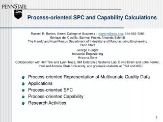
Process-oriented SPC and Capability Calculations Russell R. Barton, Smeal College of Business : rbarton@psu.edu, 814-863-7289 Enrique del Castillo, Earnest Foster, Amanda Schmitt The Harold and Inge Marcus Department of Industrial and Manufacturing Engineering Penn State George Runger Industrial Engineering Arizona State Collaboration with Jeff Tew and Lynn Truss, GM Enterprise Systems Lab, David Drain and John Fowler, Intel and Arizona State University, and graduate students at PSU and ASU Process-oriented Representation of Multivariate Quality Data Applications Process-oriented SPC Process-oriented Capability Research Activities
Process-oriented Representationof Multivariate Quality Data Define the set of n measured deviations from nominal to be a multivariate quality vector Y. Suppose that n different patterns of interest for n different process causes, say a1, a2, ... , an. If the process-oriented basis vectors a1, a2, ... , an are independent then they provide an alternative basis (or subspace if fewer than n) Y = z1a1 + z2a2 + ... + znan. A = [a1|a1| …|an] z = A-1y or z = (A'A)-1A’y
Process-oriented Representation for Chip Capacitors: Printing Registration Errors
Process-oriented Representation: Determining the Basis (characteristic signatures)
Process-oriented Representation: Standard vs Process-oriented Basis standard basis 1 0 0 0 0 0 0 0 0 1 0 0 0 0 0 0 0 0 1 0 0 0 0 0 a = e = 0 0 0 1 0 0 0 0 i i 0 0 0 0 1 0 0 0 0 0 0 0 0 1 0 0 0 0 0 0 0 0 1 0 0 0 0 0 0 0 0 1 process-oriented basis diagonal uniform differential uniform errors rotation stretch/shrink stretch/shrink stretch/shrink 1 0 1 1 -1 0 1 0 0 1 1 -1 0 1 0 1 1 0 1 1 1 0 -1 0 a = 0 1 -1 1 0 1 0 -1 i 1 0 -1 -1 1 0 1 0 0 1 -1 1 0 -1 0 1 1 0 -1 -1 -1 0 -1 0 0 1 1 -1 0 -1 0 -1 i = 1 i = 2 i = 3 i = 4 i = 5 i = 6 i = 7 i = 8
Standard Representation of y = (0, 1, 2, - 1, 0, - 1, - 2, 1)' POBREP Representation of y = (0, 1, 2, - 1, 0, - 1, - 2, 1)’ is z = (0, 0, 1, 0, 1, 0, 0, 0)’ diagonal uniform differential uniform errors rotation stretch/shrink stretch/shrink stretch/shrink Process-oriented Representation
Applications : Solder Paste Deposition Location for Processor Chip Drops of solder paste • Gonzalez-Barreto Example: • 52 leads per side • 208 solder drop volume measurements in quality vector • 5 process-oriented basis elements:
Process-oriented SPC Case 1: the common cause variation is not related to the characteristic patterns: Y = Az + e, e ~ N(0,Se) SY = Se , = (A’A)-1A’y. Case 2: the common cause variation is due solely to process-oriented basis elements: Y = AZ, Z ~ N(0,Sz) Case 3: Of course, many situations might fall between these two cases, giving: Y = AZ + e, e ~ N(0,Se), Z ~ N(0,Sz) SY = ASz,A’ + Se = (A’SY-1A)-1A’SY-1y.
Process-oriented SPC: Strategies 1. SPC using or : separate charts for each. 2. SPC using T2 or U2 applied to or : a single chart, diagnosis requires extra steps, but still more effective than T2 applied to y’s. Example: Case 3, Solder Paste Volume, Strategy 1, Sz >> Se , Var(Z5) small Z’s vs Principal Components, EWMA Chart 52 elements rather than 208 (software difficulties with Princ. Comp.)
Three univariate indices: Process-oriented Capability Cp= (USL-LSL)/6σ
Process Capability and Multivariate Capability Indices (Taam et. al (1993), Shahriari et. al (1995), Chen (1994),Wierda (1992)) Taam et al.: Assumed elliptical specifications Shahriari et al.: Presented three numbers that describe multivariate capability Chen: A general approach allowing rectangular or elliptical specifications and non-normal distributions Wierda: Direct computation of percentage conforming approach
Wierda (1993) approach to the multivariate index: • Multivariate index proposed that uses p-dimensional rectangular specification area. • Minimum expected or potentially attainable proportion of non-conformance items approach. • Original “proportion conforming” definition of capability indices is explicitly preserved • = probability of producing a good part
x2 USL2 2 LSL2 x1 1 USL1 LSL1 Wierda multivariate capability index : is a bivariate “reliability” capability measure gives multivariate proportion conforming:Integrate overbivariatenormal densityfor thedependent case Independent case: = 12
Chip capacitor: z = A-1y(Eight z’s per part) x rectangular specifications LSL < x < USL also apply to Az (since x = Az, LSL < Az < USL ) Often, covariance matrix zwill have zero non-diagonal elements—independent causes Multivariate Process-oriented Capability Example
Scenarios for computing Z matrix capability Variances forZ 1. Base 1 (Z= 0) (12, .052, .052, .052, .052, .052, .052, .052) 2. Base 1 with z1 mean shift =.5 (12, .052, .052, .052, .052, .052, .052, .052) 3. Base 1 with z1 variance increase (1.52,.052, .052, .052, .052, .052,.052, .052) 4. Base 2 (Z= 0) (12, 12, 12, .052, .052, .052, .052, .052) 5. Base 2 with z1 mean shift =.5 (12, 12, 12, .052, .052, .052, .052, .052) 6. Base 2 with z1 variance increase (1.52, 12, 12, .052, .052, .052, .052, .052) Multivariate Process-oriented Capability : Six Scenarios
Errors in Capability Estimates • Multivariate Capability Errors without POBREP (Z values) Estimated yield Estimated yield Scenario Actual yield Based on Based on Z Y 1. .94 .91 .67 2. .91 .88 .63 3. .79 .84 .50 4. .54 .59 .28 5. .51 .57 .28 6. .42 .44 .21
Process-oriented SPC and Capability Calculations Conclusions • Multivariate Capability and SPC - difficult to interpret • Process-Oriented Multivariate SPC/Capability Vectors • interpretable • practical (can be calculated with adequate precision) in many cases • efficient Acknowledgments: NSF DDM-9700330, DMI-0084909, GM Enterprise Systems Lab
Wierda (1993) multivariate indexdetails: • Compute when quality variables independent: • Compute when quality variables dependent (known): • np is MVN density • is covariance matrix • L and U are vectors of • specifications