Modularity and Community Structure in Networks*
520 likes | 771 Views
Modularity and Community Structure in Networks*. Final project *Based on a paper by M.E.J Newman in PNAS 2006. Introduction. Networks. A network: presented by a graph G(V,E): V = nodes, E = edges (link node pairs) Examples of real-life networks: social networks (V = people)

Modularity and Community Structure in Networks*
E N D
Presentation Transcript
Modularity and Community Structure in Networks* Final project *Based on a paper by M.E.J Newman in PNAS 2006
Networks • A network: presented by a graph G(V,E):V = nodes, E = edges (link node pairs) • Examples of real-life networks: • social networks (V = people) • World Wide Web (V= webpages) • protein-protein interaction networks (V = proteins)
Protein-protein Interaction Networks • Nodes – proteins (6K), edges – interactions (15K). • Reflect the cell’s machinery and signaling pathways.
Communities (clusters) in a network • A community (cluster) is a densely connected group of vertices, with only sparser connections to other groups.
Searching for communities in a network • There are numerous algorithms with different "target-functions": • "Homogenity" - dense connectivity clusters • "Separation"- graph partitioning, min-cut approach • Clustering is important for Understanding the structure of the network • Provides an overview of the network
Distilling Modules from Networks Motivation: identifying protein complexes responsible for certain functions in the cell
Important features of Newman's clustering algorithm • The number and size of the clusters are determined by the algorithm • Attempts to find a division that maximizes a modularity score Q • heuristic algorithm • Notifies when the network is non-modular
Modularity of a division (Q) Q = #(edges within groups) - E(#(edges within groups in a RANDOM graph with same node degrees))Trivial division: all vertices in one group==> Q(trivial division) = 0 ki = degree of node i M = ki = 2|E| Aij = 1 if (i,j)E, 0 otherwise Eij = expected number of edges between i and j in a random graph with same node degrees. Lemma: Eij ki*kj / M Edges within groups Q = (Aij - ki*kj/M | i,j in the same group)
Algorithm 1: Division into two groups(1) Q = (Aij - ki*kj/M | i,j in the same group) • Suppose we have n vertices {1,...,n} • s - {1} vector of size n. Represent a 2-division: • si == sj iff i and j are in the same group • ½ (si*sj+1) = 1 if si==sj, 0 otherwise • ==>
Algorithm 1: Division into two groups (2) Since B = the modularity matrix - symmetric - row sum = 0 0 is an eigvenvalue of B where
Algorithm 1: Division into two groups (3) B is symmetric B is diagonalizable (real eigenvalues) • Which vector s maximizes Q? • clearly s ~ u1 maximizes Q, but u1 may not be {1} vector • Greedy heuristic: choose s ~ u1: si= +1 if ui>0, si=-1 otherwise B's corresponding eigen vectors B's eigen values Bui = iui n=||s||2 =ai2
Example: a 2-division of a social network known group leaders known group leader Color matches the entries of the eigen vector u1: light = positive entry (si=1)dark: negative (si=-1) A network showing relationships between people in a karate club which eventually split into 2. The division algorithm predicts exactly the two groups after the split
Bij 0|1 Splitting a group ==>update Q Dividing into more than 2(1) • How to compute into more than 2? • Idea: apply the algorithm recursively on every group. =1 iff i and j are in the same group, 0 otherwise {i,j} pairs that needs to be updated in Q
Bij 0|1 Old: all the elements of g are within one group (g) New: elements of g are split into two subgroups (corresponding to s) Dividing into more than 2(2) • g - a group of ng vertices • s - a {1} vector of size ng • Compute Q for a 2-division of g
Dividing into more than 2(3) B[g] = the submatrix of B defined by g where fi(g) = sum of ith row B[g]fi({1,...,n}) = 0 generalized modularity matrix
What is [{1...5}]? Generalized modularity matrix: example g = {1, 4, 5} (1 is the minimal index)
A "generalized" 2-division algorithm (divides a group in a network)
Further techniques for modularity maximization (Combined with Neman's "generalized' 2-division algorithm)
A heuristic for 2-division The last iteration produces a 2-division which equals the initial 2-division • {g1, g2} - an initial 2-division of g • While there is an unmoved node: • Let v be an unmoved node, whose moving between g1 and g2 maximizes Q • Move v between g1 and g2 • From the ng 2-divisions generated in the previous step - let {g1, g2} be the one with maximum Q • If Q>0 ==> go to 1
Computing Q for each node Choosing j' with maximum Q moving j' and storing its Q 2.While there is an unmoved node: 1. Let v be an unmoved node, whose moving between g1 and g2 maximizes Q 2. Move v between g1 and g2
Algorithm 4 -cont. 3. From the ng 2-divisions generated in the previous step - let {g1, g2} be the one with maximum Q 4. If Q>0 ==> go to 1
Finding the leading eigen-pair The power method
The Power Method (1) • A - a diagonalizable matrix • Let (1,V1),..., (n,Vn) be n eigenpairs of A where|1| > |2| |3|... |n| • The power method finds the dominant eigenpair of A, i.e. (V1, 1) (Note that 1 is not necessarily the leading eigenvalue) • X0 = any vector. • X0 = c1V1+... +cnVn , where ci = X0Vi
The Power Method (2) • X1=AX0 = A (c1V1+... +cnVn) = c1AV1+... +cnAVn = c11V1+....+ cnnVn • X2=A2X0 = AX1= A (c11V1+....+ cnnVn) = c112V1+....+ cnn2Vn • ... • Xm=AmX0 = AXm-1= A (c11m-1V1+....+ cnnm-1Vn) = c11mV1+....+ cnnmVn ~ c1 1mV1 • If m is large enough
For simplicity, Y=Xm Power Method (3) Xm = AXm-1 = AmX0 Suppose V1Y0. For m large enough:
Power method - Example • Example: We perform only matrix-vector multiplications! Convergence usually occurs within O(n) iterations
Power method – convergence condition The desired precision To avoid numerical problems due to large numbers – normalize Xi before computing Xi+1 = A Xi X0 = X / ||X|| X1 = AX0 / ||AX0|| X2 = AX1 / || AX1|| ....
Finding the leading eigenpairusing matrix shifting • Let be the eigenvalues of A, and U1,...,Un their corresponding eigenvectors • Let ||A||1 = max |i| (exercise) • Q: What is the dominant eigenpair of A+||A||1I? • A: (1+ ||A||1, U1)
Implementation Robustness and Efficiency
Checking "positiveness" • #define IS_POSITIVE(X) ((X) > 0.00001) • Instead "x>0" ==> use IS_POSITIVE(X)
Efficient multiplications in the (extended) modularity matrix: O(n) instead O(n2) multiplication in a sparse matrix "matrix shifting" inner product f(g)ixi ("matrix shifting")
sparse_matrix_arr typedef struct{ intn; /* matrix size */ elem*values;/* the non zero elements ordered by rows*/ int*colind;/* column indices */ int*rowptr; /* pointers to where rows begin in the values array. */ } sparse_matrix_arr;
Algorithm 4 Fast score computations Computing Q for each node ==>O(n2) Computing Q for each node in O(n) before moving 1st node Updating the score AFTER a move of a node k (s is already updated)
programs computing a 2-division • sparse_mlpl < matrix_vec.in • modularity_mat <adj_matrix> <group> • spectral_div <adj_matrix> <group> <precision> • improve_div < adj_matrix> <group> <subgroup> • cluster <adj_matrix> <precision> for the power method for the power method The complete clustering algorithm (including the improvement)
Implementation process • Read and understand the document • Design ALL programs: • Data structures • Functions used by more than one program • Check your code • "Toy" examples on website - easy to debug • Your own created LARGE examples • Run your code on yeast/fly networks
Analyzing clusters in yeast and fly protein-protein interaction networks Saccharomyces cerevisiae • Input: true PPI network + 2 random networks • Task 1: infer the true network • Solution: the true network is more modular • Task 2: compute associated functions (using cytoscape + BiNGO) drosophila melanogaster
Cytoscape, BiNGO • www.cytoscape.com (version 2.5.1) • A framework for analyzing networks • Provides visualization of networks and clusters • http://www.psb.ugent.be/cbd/papers/BiNGO/ • Finding functions associated with gene cluster • Runs from cytoscape • Version 2.3 is not suitable for our project!!! (due to a bug) ==> use version 2.4 (when available) or version 2.0 (available under ~ozery/public/cytoscape-v2.5.1/plugins/BiNGO.jar).
How is the project checked? • Most checks (points): "BLACK BOX" • The common checks in "real world" • Running with fixed input files, comparing to fixed output files • Score = #(successful checks) / #(total checks) • "WHITE BOX" checks: code review (10 points maximum) • code simplicity / efficiency
A simple data structure for maintaining a division typedef struct Division_{ int n; int* group-ids; int numGroups; double Q; } Division; #nodes in the network • Complexity: • Finding all the elements of a group: O(n) • Splitting a group into 2: O(n) for each node - its group id (initially 0 - all nodes within on group)
Maintaining the generalized modularity matrix • Should we maintain the modularity matrix? • No: 1) we do not use it explicitly 2) it is a dense matrix - consumes a large memory space • Yes: 1) Despite its large size - can be kept in memory 2) Can simplify code (e.g. deriving B[g] from B, computing the L1-norm) 3) Can be used in validating the correctness of optimized multiplications (debug mode only!)
Suggestion for modules The improvement algorithm • Sparse matrices: • Data structure: sparse_matrix_lst • Reading a sparse matrix ( file / stdin) • Multiplication in a vector • Computing A[g] • Methods hiding the inner structure (allows a simple replacement of sparse_matrix_lst with another data structure for holding sparse matrices) Group Division • The generalized modularity matrix: • Data structure: A[g], k[g], M, f[g], L1-norm • Multiplication in a vector • Computing Q • printing the modularity matrix • The spectral algorithm: • 2-division • full-division
Good luck! (and have fun...)