Interconnection Networks
Interconnection Networks. Interconnection Networks. Bus-oriented Ring Crossbar Two and Three dimensional mesh Multi-level switched Hypercube. General Issues. n − to − n networks connect PE ’ s directly n − by − n PE ’ s are interconnected through a network of switches.


Interconnection Networks
E N D
Presentation Transcript
Interconnection Networks • Bus-oriented • Ring • Crossbar • Two and Three dimensional mesh • Multi-level switched • Hypercube
General Issues • n − to − n networks connect PE’s directly • n − by − n PE’s are interconnected through a network of switches. • functional entities: paths and switches. • A path is composed of one or more links and switches. • A switch routes a message through one of several alternative paths. • dedicated paths can be unidirectional point-to-point and bidirectional point-to-point. • shared paths are bidirectional paths that visit more than 2 nodes.
General Issues • transfer strategies • direct: no switching elements between nodes • indirect: one or more switching elements between nodes • centralized transfer - control of switches is centralized • decentralized transfer - control is distributed among a number of switching elements
General issues • Modes of operation: • Synchronous • asynchronous, and • combined.
Performance factors • connectivity: or degree of a node refers to the number of nodes that can be reached in one hop. • Bandwidth: total number of messages delivered per unit of time. • Latency: a measure of the overhead involved in transmitting a message over the network from source to destination. Typically defined as the time required to transmit a zero- length message.
Performance factors • Average distance: number of links in the shortest path between two nodes: • Nd is the number of nodes at distance d apart. r is the diameter of the network obtained as the maximum of the minimum distances between all pair of nodes. N is the number of nodes.
Performance Factors • Normalized distance - It is desirable to have a low average distance. However, it results in high degree nodes which it is expensive. A normalized distance is then defined as: • where P is the number of communication ports per node.
Performance Factors • Regularity - IN’s have a regular pattern that can be repeated to form larger networks. • cost modularity - incremental hardware cost. • place modularity – measure of expandability in terms of how easy the network can be expanded by adding new nodes.
Routing Protocols • Circuit switching • a path is first established between source and destination nodes; then the message is transmitted. Suitable for large messages.
Routing Protocols • Packet switching • Messages are divided into units called packets • packets are routed in a stored and forward manner. At each intermediate node the packet is buffered and then forwarded to the next link based on its destination address. • packets may arrive at the destination in a random order where they are reassembled • suitable for short messages • switches are more complex because of the buffering requirements.
Store-and-Forward • Utilizing this method, a switch reads an entire frame into an internal buffer. It then examines the MAC address. It compares the MAC address against an internal table of addresses which tells the device which MAC addresses are on each interface. Once it has the interface identified, it sends the frame out that interface. The advantage to this method is that corrupted frames are identified and discarded without being forwarded. The disadvantage is that a great deal of buffer memory is required to store frames arriving on busy interfaces. Most modern switches are so fast that they use store and forward exclusively.
Cut-Through • With this method, the switch only examines enough of a frame to determine the destination MAC address. It then establishes a connection to the interface through which that address can be reached and the frame is sent out. The advantage of this method is very fast operation. The disadvantage is that corrupted frames will be forwarded.
Routing Protocols • Wormhole switching (cut-through routing) • combination of circuit and packet switching • messages are broken into small units called flits (flow control digits). • all flits follow the same route to the destination • the leading flit sets the switches in the path; the remaining flits follow. Store and forward buffering overhead is reduced.
Wormhole • Wormhole routing is a system of simple routing in computer networking based on known fixed links, typically with a short address. The name plays on the way packets are sent over the links: the address is so short that it can be translated before the message itself arrives. This allows the router to quickly set up the routing of the actual message and then "bow out" of the rest of the conversation. • Wormhole routing is primarily used in multiprocessor systems, notably hypercubes . In a hypercube computer each CPU is attached to several neighbors in a fixed pattern, which reduces the number of hops from one CPU to another. Each CPU is given a number (typically only 8 to 16-bit ), which is its network address, and messages to CPUs are sent with this number in the header. When the message arrives at an intermediate CPU for forwarding, the CPU examines the header (very quickly), sets up a circuit to the next CPU, and then bows out of the conversation. In this way the messages rarely (if ever) have any delay as they travel though the network, so the speed is similar to the speed at which the computers would function if they were directly connected.
Routing mechanisms • Static routing (deterministic) • based on the network topology a unique path is established between source and destination. Since it ignores the state of the network, results in an uneven use of the network causing traffic congestion. • Dynamic routing • the path established is based on the state of the network. Thus, heavily used links or nodes are avoided.
Topologies • Static: links between two nodes are dedicated paths. Interconnections are derived analytically in terms on the communication patterns required by the applications. • Dynamic: interconnection patterns change as computation progresses. Switches are set to reconfigure the routing required.
Topologies- Static • One-dimensional • Each node is connected to a neighbouring node • For linear array there are boundary nodes. • Links can be unidirectional or bi-directional • Nodes receive messages and forward them if not for them. • Logical complexity is low.
Topologies • Bus networks • The simplest topology but with the highest potential contention and lowest performance. Each processor is connected to a common bus but all share global memory which is also connected to the common bus. Fig. 6.3 [Sto93]
Topologies • Commercial bus-based multiprocessors support as many as 32 microprocessors. Larger num- ber of microprocessors leads to degraded performance (technology factor: stray capacitance because of metal wiring introduce noise and limit bandwidth). In fact: • Bus bandwidth decreases as N (No. of processors) grows. (crosstalk increases). • Bus bandwidth as a function of connection length is greater in short buses than than the bandwidth of long buses. • Options: reduce number of processors, physical size of components (expensive!), change technology (i.e., optical buses).
Topologies • In SIMD systems loop networks transfer messages between PE’s simultaneously in a lock-step mode. • Transfer of messages is controlled by the CP through SHIFT and ROTATE instructions. • the Std. IEEE 802.5 turns the loop into a logical bus. The transmitting processor holds a “token” to send a message to the ring which acts like a bus and the remaining processors listen. • the “token” is a combination of signals that circulate in the ring. When a processor is ready to transmit a message, grabs the token, transmits the message and releases the token.
Topologies • delay increases linearly with the number of processors in the ring. This delay is introduced by each processor that repeats incoming messages. This can be made equivalent to the delay between stages in a pipelined structure. By overlapping transmissions with computations the effective bandwidth can be fully utilized. • Technology: because of the short length interconnections, this topology is well suited for VLSI implementation (on-chip clock rate 200 MHz.). With optical connections speeds on the order of 1 GHz are possible.
Topologies • Unidirectional one-dimensional ring networks fail when any one link is broken. • Bidirectional, two link failures partitions the network into two disconnected parts. • Can add redundant paths for fault tolerance, chordal ring is an example
Topologies • Near-neighbor mesh . Examples: Illiac IV, MPP, ICL Distributed array processors, IBM Wire routing machine. Fig. 2-9 [Sie90]. • Nodes are arranged in a matrix form. Regularity of interconnections and locality of interactions among PE’s, makes this topology attractive for several specific applications.
Topologies • Each node is connected to four of its neighbors. • Max network latency = N • No direct synchronization and global communication is supported. • performance will depend on the proportion of global operations required. • Note that in the worst case the longest communication path is for a mesh of N processors. The average in a torus-type connection is
Topologies • Check the Illiac IV interconnection as an example:
Topologies • Crossbar networks. Fig. 5.14, Fig. 6.6 [Sto93] • connect any PE to any other free PE any time; highest performance; highest cost. • the most expensive (O(N 2 )) and with the highest complexity. Only feasible for small N . • it offers the least contention as each PE can be connected to each memory module directly. Up to N simultaneous accesses are possible. Contention will occur only if more than two accesses are attempted to the same module.
Topologies – Two-dimensional • Binary Trees • Each interior node has a degree of 3. Leaves have a degree of 1. The root node has degree of 2 • Routing is simple: a source node finds a destination node by ascending the tree until reaching the ancestor of the destination node; then the message descends until it reaches its destination. • Latency O(log2N )
Topologies • Complete interconnection Fig. 5.12
Topologies (completely connected) • each node is connected to every other node, i.e., each node has a degree of N − 1. There are N (N − 1)/2 links. Consequently the minimal length path contains only one link. • routing is trivial. Each node should be able to receive messages on a multiplicity of paths. • scalable? to add one node implies N extra links and all nodes must have an additional port. Thus, it is costly and place modularity is low
Topologies • Hypercube Fig. 5.13
Topologies (hypercube) • multidimensional near-neighbor netk. A k-dimensional cube (k-cube) contains 2k nodes, each of degree k. • nodes can be identified using k-bits and the labels of each neighboring node differ only in one bit position. • the number of different bits in the labels of source and destination nodes determine the number of hops needed to reach the destination node.
Topologies (hypercube) • routing is simple: For a k-cube, the routing algorithm takes at most k steps. At step i the message is routed to an adjacent node with the ith bit flipped. Example: source node = 00000 and dest. node = 01110 → three possible routes. Message is sent to 00010 then send to 00110, and finally send to 01110 • Latency is O(log2 N ) • the number of nodes must be a power of two. To scale implies poor cost and low place modularity.
Quicksort Very popular sequential sorting algorithm that performs well with average sequential time complexity of O(nlogn). First list divided into two sublists. All numbers in one sublist arranged to be smaller than all numbers in other sublist. Achieved by first selecting one number, called a pivot, against which every other number is compared. If the number is less than the pivot, it is placed in one sublist. Otherwise, it is placed in the other sublist. Pivot could be any number in the list, but often first number in list chosen. Pivot itself could be placed in one sublist, or the pivot could be separated and placed in its final position.
Parallelizing Quicksort Using tree allocation of processes
Analysis Fundamental problem with all tree constructions – initial division done by a single processor, which will seriously limit speed. Tree in quicksort will not, in general, be perfectly balanced Pivot selection very important to make quicksort operate fast.
Hypercube Quicksort Hypercube network has structural characteristics that offer scope for implementing efficient divide-and-conquer sorting algorithms, such as quicksort.
Complete List Placed in One Processor Suppose a list of n numbers placed on one node of a d-dimensional hypercube. List can be divided into two parts according to the quicksort algorithm by using a pivot determined by the processor, with one part sent to the adjacent node in the highest dimension. Then the two nodes can repeat the process.
Example 3-dimensional hypercube with the numbers originally in node 000: Finally, the parts sorted using a sequential algorithm, all in parallel. If required, sorted parts can be returned to one processor in a sequence that allows processor to concatenate sorted lists to create final sorted list.
Hypercube quicksort algorithm - numbers originally in node 000
Hypercube numbers distributed to begin with Note the degree decrease of the partial hypercube after each phase.
Switching networks • Switching networks offer a cost/performance compromise between two extremes, • Bus networks • Cross-bar networks.
Bus Network • Simple to build • Low cost • Lowest performance
Crossbar Network • Multiple simultaneous communications • Least amount of contention • High cost