Download
1 / 10
100 likes | 237 Views
Commuting patterns and Firm Decentralization. Introduction This paper written by Robin Dubin exams commuting patterns of employed individuals and firm decentralization by testing the monocentric model.

E N D
Commuting patterns and Firm Decentralization Introduction • This paper written by Robin Dubin exams commuting patterns of employed individuals and firm decentralization by testing the monocentric model. • By examining the monocentric model, the paper will show us how sex, income, race, household responsibilities, residential and job mobility determine commuting behavior as firms decentralize.
Monocentric model Most employed individuals must travel between home and work on a daily basis, work place commuting thus has provided the point of departure for the monocentric model of residential location. In the monocentric situation, all employment is located at the central business district; decentralized firm location enables workers to shorten their commutes as firms have left the central business district, to move into the residential area. One of the major behavioral assumptions of the monocetric model is that comsumers prefer less commuting to more. Hence the model predicts that workers will take advantage of firm decentralization. • Assumption (a) The employees are willing to move in order to be near the new suburban location (people prefer less commuting) (b) The firm’s employees are located in one portion of the city so that the firm can locate nearer to them by suburbanizing; (c) the firm can change employees and thereby employ people who live near the new location.
Discussion • Suppose homogeneous jobs, workers and housing,all employment is located in the central business district. If a firm suburbanized, in the very short run, total commuting in the city will increase. But two adjustments reduce commuting: workers can follow the firm, and the company can hire new workers that live near the new location. Commuting will reduce eventually. • More realistically, workers differ by incomes, preferences or training; Jobs differ by skill requirements, and the housing stock is not homogeneous. Workers are not indifferent among all residential sites and thus may very well be unwilling to move even if such moves reduce commuting costs. If workers are reluctant to change houses or jobs, decentralization may increase, rather than decrease, total commuting! • Individuals’ income, job characteristics, residential characteristics and some other factors may have some effect on determining their commuting patterns.
Empirical Model The monocentric model is based on a separation of the house and work place. Therefore, this separation can be measured either in terms of commuting time(T) or distance(D). • Monocentric vs. Actural commuting ΔD(Δ T)= HYP – ACTUAL where _ ΔD (Δ T) is the distance (or time) the worker would have to travel if he were employed in the CBD minus the atural commute _HYP is hypothetical monocentric commute( in miles or minutes) _ ACTURAL is actual commute (in miles or munites) If the commute is shorter in the presence of suburbanization, ΔD(ΔT) will be positive, which is predicted by monocentric model; If the worker commute farther than he would if his job were located in CBD, then suburbanization has increased his commute, and ΔD(ΔT) will be negative.
Actual commuting ACTUAL= 0 + OPT + 1HDEQ + 2JDEQ + U1 Where OPT is optimal commute (not directly observed) HDEQ is residential location disequilibrium factor (ndo) JDEQ is employment location disequilibrium factor (ndo) U is random, unexplained disturbances Optimal commuting OPT = δ0 +δ1BEN + δ2COST +δ3 F + U2 Where BEN is the benefit of commuting an additional mile COST is the cost of commuting an additional mile F is number of full-time workers in household
Commuting Benefit BEN= λ0 + λ1PCHILD + λ2Y +U3 Where PCHILD =0 if no children under 12, =1 otherwise Y is household income (annual income in hundreds of dollars) Commuting cost COST= θ0 + θ1Y + θ2MODE +θ3 HR +U4 Where MODE is transportation mode (0= auto, 1= bus) HR is household responsibilities (not directly observed) Household responsibilities HR = ρ0 + ρ1PCHILD +ρ2NADULT + ρ3F + ρ4SEX + U5 Where NADULT is number of household members older than eighteen SEX = 0 for male, =1 for female
Residential disequilibrium HDEQ= α0 +α1OWNRNT + α2L + α3RACE + α4PCHILD + α5Y + U6 Where OWNRNT is residential tenure (0= own, 1=rent) L is length of time at current location (1=< 6mos., 2=7-12 mos., 3=13-24 mos., 4=> 2 yrs.) Race =0 for White, =1 for Black Job disequilibrium JDEQ= γ0 +γ1 Y+γ2TEN +γ3 TS +γ4 RACE +γ5SEX + U7 Where TEN is job tenure TS is dummy variable representing job skills that are highly transferable (1=service or sales workers, 0= any other occupation)
Hypothetical monocentric commute HYP = μ0 +μ1 PCHILD+μ2 Y+μ3 JDIST+ U8 Where JDIST is distance of job from the CBD ΔD (ΔT)=П0+ П1Y +П2 MODE +П3 PCHILD +П4 NADULT +П4 F +П5 OWNRENT +П7 L+П8 RACE+П9 SEX+П10 TS+П11 JDIST +П12 TEN+ε ~ The expected signs on the Пi can be derived from the expected signs on the coefficients of the structural equations. ~ The coefficients for SEX, TS, OWNRENT, MODE and JDIST are expected to be positive. This means that women, workers with highly transferable job skills, renters, public transit users, and workers whose jobs are located far from the CBD are all expected to use firm decentralization to shorten their commutes.
~ Coefficients of Race, NADULT, L, AND TEN are all expected to have negative coefficients. Being black, having more adults in the household and having longer residential or job tenure should adversely affect a worker’s ability to take advantage of firm decentralization. ~ Coefficients of Y, PCHILD, and F can’t be determined. Because high income workers located far away from CBD, but also have a high cost to change their job, they affect ΔD(ΔT) in opposite ways. Regarding PCHILD, the relationship between the presence of children and residential mobility is unknown. Finally for F, increased household responsibilities increase ΔD(ΔT), while the difficulty of optimizing with respect to two or more work places reduces it.