Download

1 / 70
700 likes | 884 Views
Pattern Formation in a Reaction-diffusion System. Noel R. Schutt, Desiderio A. Vasquez Department of Physics, IPFW, Fort Wayne IN. Turing patterns in a modified Lotka-Volterra model. Turing Patterns. Predicted by Alan Turing in 1952 Patterns in chemical/biological systems

E N D
Pattern Formation in a Reaction-diffusion System Noel R. Schutt, Desiderio A. Vasquez Department of Physics, IPFW, Fort Wayne IN
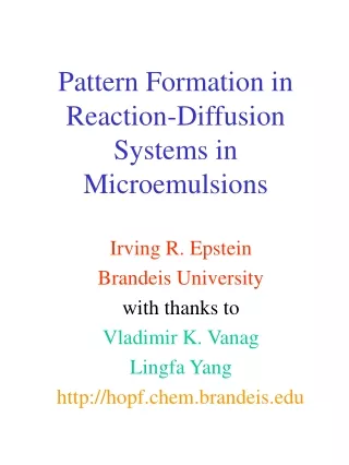
Turing Patterns • Predicted by Alan Turing in 1952 • Patterns in chemical/biological systems • Non-homogenous solutions to DE
Turing Patterns Phys Rev Lett 64 (1990) 2953 Castets, Dulos, Boissonade, De Kepper
Turing Patterns http://chaos.utexas.edu/research/spots/spots.html
Lotka-Volterra Model x: Prey or Activator y: Predator or Inhibitor Introduction to Ordinary Differential Equations Stephen Sapesrtone
Lotka-Volterra Model http://mathworld.wolfram.com/Lotka-VolterraEquations.html
Modified Lotka-Volterra Model • Change from a single value to one dimension of space • Add diffusion • Add intraspecies interaction term
Modified Lotka-Volterra Model • Now patterns can develop • In 2005 patterns were found in this model in one dimension • Use finite difference equation to Reproduce results
How to solve the equation • To reduce the runtime, use an implicit Euler method for time • Space is in a 321x321 grid
How to solve the equation • Original math code in FORTRAN • Math code is fairly simple • Perl wrapper code to simplify working with math code • php code to organize results • Results take 20MB to 2.8GB per run
Initial conditions • Solve equation for steady states • Each set of values gives three steady states e.g. 7.99 (unstable), 11.48 (unstable), 22.22 (stable) • Filled the grid with this value ± small disturbance
Development - X x0=14
Development - Y x0=14
X Y 9 holes x0=14
X Y 9 holes x0=15
X Y 8 holes
A 3 holes
B 4 holes
A 1/10 x0=44a
A 2/10 x0=44a
A 3/10 x0=44a
A 4/10 x0=44a
A 5/10 x0=44a
A 6/10 x0=44a
A 7/10 x0=44a
A 8/10 x0=44a
A 9/10 x0=44a
A 10/10 x0=44a
B x0=44b
C x0=44c
A x0=45a
B x0=45b
C x0=45c