Download

1 / 26
270 likes | 402 Views
Seasonal changes in biosphere-atmosphere carbon exchange influence atmospheric CO 2 concentration. Marine primary production and the global carbon cycle. What limits marine production?. Water? (no, except intertidal)

E N D
Seasonal changes in biosphere-atmosphere carbon exchange influence atmospheric CO2 concentration
What limits marine production? • Water? (no, except intertidal) • Strong contrast with terrestrial systems, where water is the dominant limiting factor • CO2? (no, except sometimes intertidal) • CO2-bicarbonate-carbonate equilibrium supplies CO2 • Light? (always at depth) • Nutrients? (usually)
Ocean currents create radically different environments Centers of gyres have little mixing Off-shore currents cause upwelling Warm oceans have high vertical stability (not much vertical mixing, thus low nutrients!)
Euphotic zone of oceans are frequently nutrient poor – spatial separation of light and nutrients –Terrestrial plants overcome this via vascular transport Some phytoplankton swim or alter buoyancy to reduce nutrient limitation Nutrient concentrations of euphotic zone are highest in upwelling currents Always depleted at surface by algal uptake
Latitudinal gradients in productivity • Polar oceans are most productive • More effective mixing of nutrients from depth because of lower surface T, and weaker vertical T gradient • Polar lands are least productive • Less rapid nutrient release from SOM • Consequences • Bipolar bird, fish and mammal migrations to capitalize on spring blooms of phytoplankton • Polar distribution of anadromous fish (eat marine, breed fresh)
Major upwelling zones off Peru, Africa Outer Banks, North Pacific California, North Africa Wind-mixing off Antarctica
Marine Primary Production • Production is highest in continental margins and shallow seas, because – Upwelling transports nutrients to the surface – Nutrient runoff from land
• Production is low in ‘blue water’, the open ocean. – Nutrient availability is low in some areas of the open ocean– But in others, there are vast expanses of areas with high nutrients (N and P) but low chlorophyll (i.e., low NPP)– These are called HNLC (“High Nutrient, Low Chlorophyll”) zones– They occur in about 1/5th of the world’s oceans, including the Southern Ocean, Equatorial and subarctic North Pacific
Oceanographers hypothesized that zooplankton grazers were so active in these areas, that they kept populations of phytoplankton low But there was no evidence for this idea. In 1981, John Martin began to tackle this “mystery of the desolate zones” He speculated that iron could be responsible Up until then, measuring trace [Fe] had been verydifficult, but new, more precise methods by the 80smade it possible to make these measurementsaccurately Martin measured [Fe] in the HNLC zones, and found it to be exceedingly low, or non-existent (below detection limits)
The phytoplankton in the iron-dosed jar flourished after a few days. In Antarctica, Martin’s team collected clean water and added iron to some samples and left others untreated. The samples were placed in baths on the deck of the ship. (Graph courtesy U.S. Joint Global Ocean Flux Study, based on data from K. Johnson and K. Coale.)
“Give me half a tanker filled with iron, and I’ll give you another ice age” John Martin (1989) Claimed that iron levels could in part be responsible for past ice ages During an ice age much of the fresh water on the continents is locked up in the ice caps, and the exposed landmasses become drier than they are today. If large amounts of iron were swept off these arid landmasses by wind and dumped into the ocean's “desolate zones,” the resulting growth of phytoplankton would effectively pump vast amounts of carbon dioxide from the atmosphere deep into the seas. What does the ice core record show?
Dust Atm CO2 From the ice core record, dust inputs are correlated with oceanic productivity over the past several hundred thousand years: dust deposition (Fe inputs) is correlated with depletion of atmospheric CO2 dust deposition is also correlated with the accumulation of organic carbon in ocean sediments
Large-scale, open-ocean experiments: the true test of the iron hypothesis During the 1993 Iron Enrichment Experiment (IRONEX), researchers dumped iron into a 64-square-kilometer area and measured the response of phytoplankton. The photograph above shows researchers at the Naval Postgraduate School preparing iron to be dumped in the sea.
Monitoring CO2 levels in the water showed increasedphotosynthetic activity where the iron had been released
But the results were truly dramatic, as reported in Science News, 148:220 (1995), “Nothing had prepared them for the color of the water. The oceanographers watched in awe as the R. V. Melville pliedPacific waves dyed a soupy green by a bumper crop of tinyocean plants. The tint was abnormal. Only a day before, this patch of water near the Galapagos Islands had sparkled with electric blue clarity, a quality owing to the general absence or phytoplankton. They had transformed this marine desert into a garden simply by sprinkling a dilute solution of iron into the water.”
The results of the Southern Ocean Iron Enrichment Experiment (SOIREE) experiment in 1999 were captured by the Sea-viewing Wide Field-of-view Sensor (SeaWiFS). The bright comma in the image indicates phytoplankton growth stimulated by iron added during the course of the experiment.(Image courtesy Jim Acker, Goddard Distributed Active Archive Center, the SeaWiFS Project, NASA/Goddard Space Flight Center, and ORBIMAGE
+ Fe + NPP + Ocean carbon storage Atmospheric[CO2] ??? “We have demonstrated that we have the key now for turningthis system on and off. I think some will be encouraged bythese findings. Therein lies the dilemma.” Kenneth Coale, lead scientist in the IRONEX experiments
Another possible, ‘geoengineering’ fix… deep ocean CO2 injection Recall that, of the global reservoirs of C, the deep ocean is the second largestCO2 in the deep ocean has a very slow turnover time, many thousands of years (longer than wood or soil) But delivery to the deep ocean by physical dissolution and oceantransport is quite slow So, why not speed up this natural process, by directly injecting pure liquid CO2 into deep ocean waters???
Would it stay there? very likely, yes Is it economically feasible? under investigation! What would the environmental impacts be? pH changes in the ocean very large changes locally (near sites of injection) could occur on a worldwide scale
Potential Impacts of Deep Ocean CO2 Injection: ecosystems at such depths are very to changes in biogeochemistry particularly to changes in pH that surely would result from such large infusions of CO2 Seibel and Walsh (2001) estimate that sequestration of enough atmospheric CO2 to stablilize atmospheric concentrations at 550 ppm (twice the pre-industrial level) would decrease ocean pH globally by about 0.1 by 2100. The pH goes down due to the formation of carbonic acid: H2O + CO2 H2CO3 (carbonic acid) Because of the high sensitivity of most deep-sea organisms to rapid changes in pH, such massive CO2 disposal likely would have significant adverse consequences on deep-sea ecosystems. Reference Seibel, B. A., and P. J. Walsh,, 2001: Potential impacts of CO2 injection on deep-sea biota. Science 294, 319-320.
Simulated time evolution of pH contours near the CO2 injection point - background current velocity: 5 cm/s- liquid CO2 droplet initial radius (as injected): 7 mm- liquid CO2 injection mass flow rate: 1 kg/s The pH scale ranges from 5.9 to 7.9, increasing in 0.2 increments. The background pH (shown in red) was taken as 8.0. After approximately 45 minutes, the plume reaches a steady state within 100 m of the CO2 release point. Local changes in pH will be even larger…
What do you think? Should we fertilize with iron? Why or why not? Should we inject CO2 into the oceans, into oil fields, saline beds…??? Why or why not?