Graphical models, belief propagation, and Markov random fields
1.01k likes | 1.03k Views
This article explores the concepts of graphical models and belief propagation, illustrating how tinker toys can build complex probability distributions. It delves into steps for building graphical models, the derivation of belief propagation, and optimal solutions for different scenarios. The text covers the importance of modularity in probabilistic graphical models and provides a toy example to aid comprehension.

Graphical models, belief propagation, and Markov random fields
E N D
Presentation Transcript
Graphical models, belief propagation, and Markov random fields Bill Freeman, MIT Fredo Durand, MIT 6.882 March 21, 2005
Color selection problem • (see Photoshop demonstration)
L R Squared difference, (L[x] – R[x-d])^2, for some x. d Stereo problem x Showing local disparity evidence vectors for a set of neighboring positions, x. d
Super-resolution image synthesis How select which selection of high resolution patches best fits together? Ignoring which patch fits well with which gives this result for the high frequency components of an image:
Things we want to be able to articulate in a spatial prior • Favor neighboring pixels having the same state (state, meaning: estimated depth, or group segment membership) • Favor neighboring nodes have compatible states (a patch at node i should fit well with selected patch at node j). • But encourage state changes to occur at certain places (like regions of high image gradient).
x1 x2 x3 y z Graphical models: tinker toys to build complex probability distributions • Circles represent random variables. • Lines represent statistical dependencies. • There is a corresponding equation that gives P(x1, x2, x3, y, z), but often it’s easier to understand things from the picture. • These tinker toys for probabilities let you build up, from simple, easy-to-understand pieces, complicated probability distributions involving many variables. http://mark.michaelis.net/weblog/2002/12/29/Tinker%20Toys%20Car.jpg
Steps in building and using graphical models • First, define the function you want to optimize. Note the two common ways of framing the problem • In terms of probabilities. Multiply together component terms, which typically involve exponentials. • In terms of energies. The log of the probabilities. Typically add together the exponentiated terms from above. • The second step: optimize that function. For probabilities, take the mean or the max (or use some other “loss function”). For energies, take the min. • 3rd step: in many cases, you want to learn the function from the 1st step.
A more general compatibility matrix (values shown as grey scale)
y1 x1 y2 x2 y3 x3 Derivation of belief propagation
y1 y3 y2 x1 x3 x2 The posterior factorizes
y1 y3 y2 x1 x3 x2 Propagation rules
y1 y3 y2 x1 x3 x2 Propagation rules
y1 y3 y2 x1 x3 x2 Propagation rules
Belief propagation: the nosey neighbor rule “Given everything that I know, here’s what I think you should think” (Given the probabilities of my being in different states, and how my states relate to your states, here’s what I think the probabilities of your states should be)
Belief propagation messages A message: can be thought of as a set of weights on each of your possible states To send a message: Multiply together all the incoming messages, except from the node you’re sending to, then multiply by the compatibility matrix and marginalize over the sender’s states. = i j j i
Beliefs To find a node’s beliefs: Multiply together all the messages coming in to that node. j
x1 x2 x3 x1 x2 x3 Simple BP example y1 y3
x1 x2 x3 • To find the marginal probability for each variable, you can • Marginalize out the other variables of: • Or you can run belief propagation, (BP). BP redistributes the various partial sums, leading to a very efficient calculation. Simple BP example
Belief, and message updates j = i j i
Optimal solution in a chain or tree:Belief Propagation • “Do the right thing” Bayesian algorithm. • For Gaussian random variables over time: Kalman filter. • For hidden Markov models: forward/backward algorithm (and MAP variant is Viterbi).
Making probability distributions modular, and therefore tractable:Probabilistic graphical models Vision is a problem involving the interactions of many variables: things can seem hopelessly complex. Everything is made tractable, or at least, simpler, if we modularize the problem. That’s what probabilistic graphical models do, and let’s examine that. Readings: Jordan and Weiss intro article—fantastic! Kevin Murphy web page—comprehensive and with pointers to many advanced topics
A toy example Suppose we have a system of 5 interacting variables, perhaps some are observed and some are not. There’s some probabilistic relationship between the 5 variables, described by their joint probability, P(x1, x2, x3, x4, x5). If we want to find out what the likely state of variable x1 is (say, the position of the hand of some person we are observing), what can we do? Two reasonable choices are: (a) find the value of x1 (and of all the other variables) that gives the maximum of P(x1, x2, x3, x4, x5); that’s the MAP solution. Or (b) marginalize over all the other variables and then take the mean or the maximum of the other variables. Marginalizing, then taking the mean, is equivalent to finding the MMSE solution. Marginalizing, then taking the max, is called the max marginal solution and sometimes a useful thing to do.
To find the marginal probability at x1, we have to take this sum: If the system really is high dimensional, that will quickly become intractable. But if there is some modularity in then things become tractable again. Suppose the variables form a Markov chain: x1 causes x2 which causes x3, etc. We might draw out this relationship as follows:
But if we exploit the assumed modularity of the probability distribution over the 5 variables (in this case, the assumed Markov chain structure), then that expression simplifies: P(a,b) = P(b|a) P(a) By the chain rule, for any probability distribution, we have: Now our marginalization summations distribute through those terms:
Belief propagation Performing the marginalization by doing the partial sums is called “belief propagation”. In this example, it has saved us a lot of computation. Suppose each variable has 10 discrete states. Then, not knowing the special structure of P, we would have to perform 10000 additions (10^4) to marginalize over the four variables. But doing the partial sums on the right hand side, we only need 40 additions (10*4) to perform the same marginalization!
Another modular probabilistic structure, more common in vision problems, is an undirected graph: The joint probability for this graph is given by: Where is called a “compatibility function”. We can define compatibility functions we result in the same joint probability as for the directed graph described in the previous slides; for that example, we could use either form.
y1 y3 y2 x1 x3 x2 Y ( x , x ) 1 3 No factorization with loops!
Justification for running belief propagation in networks with loops Kschischang and Frey, 1998; McEliece et al., 1998 • Experimental results: • Error-correcting codes • Vision applications • Theoretical results: • For Gaussian processes, means are correct. • Large neighborhood local maximum for MAP. • Equivalent to Bethe approx. in statistical physics. • Tree-weighted reparameterization Freeman and Pasztor, 1999; Frey, 2000 Weiss and Freeman, 1999 Weiss and Freeman, 2000 Yedidia, Freeman, and Weiss, 2000 Wainwright, Willsky, Jaakkola, 2001
i Region marginal probabilities i j
Belief propagation equations Belief propagation equations come from the marginalization constraints. i i j = i j i
Results from Bethe free energy analysis • Fixed point of belief propagation equations iff. Bethe approximation stationary point. • Belief propagation always has a fixed point. • Connection with variational methods for inference: both minimize approximations to Free Energy, • variational: usually use primal variables. • belief propagation: fixed pt. equs. for dual variables. • Kikuchi approximations lead to more accurate belief propagation algorithms. • Other Bethe free energy minimization algorithms—Yuille, Welling, etc.
Update for messages Kikuchi message-update rules Groups of nodes send messages to other groups of nodes. Typical choice for Kikuchi cluster. i j i j = i j i = k l Update for messages
Generalized belief propagation Marginal probabilities for nodes in one row of a 10x10 spin glass BP: belief propagation GBP: generalized belief propagation ML: maximum likelihood
References on BP and GBP • J. Pearl, 1985 • classic • Y. Weiss, NIPS 1998 • Inspires application of BP to vision • W. Freeman et al learning low-level vision, IJCV 1999 • Applications in super-resolution, motion, shading/paint discrimination • H. Shum et al, ECCV 2002 • Application to stereo • M. Wainwright, T. Jaakkola, A. Willsky • Reparameterization version • J. Yedidia, AAAI 2000 • The clearest place to read about BP and GBP.
Probability models for entire images: Markov Random Fields • Allows rich probabilistic models for images. • But built in a local, modular way. Learn local relationships, get global effects out.
MRF nodes as pixels Winkler, 1995, p. 32
MRF nodes as patches image patches scene patches image F(xi, yi) Y(xi, xj) scene
Network joint probability 1 Õ Õ = Y F P ( x , y ) ( x , x ) ( x , y ) i j i i Z , i j i scene Scene-scene compatibility function Image-scene compatibility function image neighboring scene nodes local observations
In order to use MRFs: • Given observations y, and the parameters of the MRF, how infer the hidden variables, x? • How learn the parameters of the MRF?
Outline of MRF section • Inference in MRF’s. • Iterated conditional modes (ICM) • Gibbs sampling, simulated annealing • Variational methods • Belief propagation • Graph cuts • Vision applications of inference in MRF’s. • Learning MRF parameters. • Iterative proportional fitting (IPF)
Iterated conditional modes • For each node: • Condition on all the neighbors • Find the mode • Repeat. Described in: Winkler, 1995. Introduced by Besag in 1986.
Outline of MRF section • Inference in MRF’s. • Iterated conditional modes (ICM) • Gibbs sampling, simulated annealing • Variational methods • Belief propagation • Graph cuts • Vision applications of inference in MRF’s. • Learning MRF parameters. • Iterative proportional fitting (IPF)
Gibbs Sampling and Simulated Annealing • Gibbs sampling: • A way to generate random samples from a (potentially very complicated) probability distribution. • Simulated annealing: • A schedule for modifying the probability distribution so that, at “zero temperature”, you draw samples only from the MAP solution. Reference: Geman and Geman, IEEE PAMI 1984.
3. Sampling draw a ~ U(0,1); for k = 1 to n if break; ; Sampling from a 1-d function • Discretize the density function 2. Compute distribution function from density function
x2 x1 Gibbs Sampling Slide by Ce Liu
Gibbs sampling and simulated annealing Simulated annealing as you gradually lower the “temperature” of the probability distribution ultimately giving zero probability to all but the MAP estimate. What’s good about it: finds global MAP solution. What’s bad about it: takes forever. Gibbs sampling is in the inner loop…