Dual frequency interferometry and phase transfer at the Submillimeter Array
330 likes | 345 Views
This summary highlights the operational details and calibration challenges faced by the Submillimeter Array (SMA). It emphasizes the need for strong gain calibrators at high frequencies for accurate interferometry. The text delves into the instrumental setup, frequency bands, and potential sources for calibration at 690 GHz. It also discusses phase transfer techniques and observational strategies involving masers and known sources. The proposed calibration method involves comparing phase and amplitude relationships between different frequency bands using strong continuum sources.

Dual frequency interferometry and phase transfer at the Submillimeter Array
E N D
Presentation Transcript
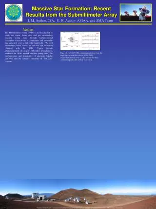
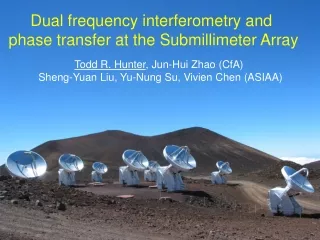
Dual frequency interferometry and phase transfer at the Submillimeter Array Todd R. Hunter, Jun-Hui Zhao (CfA) Sheng-Yuan Liu, Yu-Nung Su, Vivien Chen (ASIAA)
Summary of present SMA operations Antennas: 8, diameter 6m, surface rms: 12 to 20 microns Baselines: 28, from 16m to 500m (angular scales 0.3” to 15” @ 345 GHz) Receivers: DSB, 1-polarization, 3 bands: 180-245, 260-355, 620-695 GHz Correlator: 2 GHz BW per SB: 3072 channels x 2 sidebands x 2 receivers Next proposal deadline: March 2006 (http://sma1.sma.hawaii.edu)
Lack of Strong Gain Calibrators at High-Frequency Interferometry requires calibration of antenna-based phase & amplitude introduced by instrumental and atmospheric effects. SMA sensitivity: Tsys ~ 100 K at 230 GHz (10 mJy in 5 min) (6-antennas) Tsys ~ 2000 K at 690 GHz (200 mJy in 5 min) For good phase solutions, we need S/N > 10 per baseline This requires a strong source! { 0.5 Jy at 230 GHz (70 quasars with F > 1Jy) 8 Jy at 690 GHz (maybe 2 or 3 quasars) Quasars are inadequate for the SMA at 690 GHz
Other options in 690 GHz band: Minor planets Typical flux density Typical 230 GHz658 GHzDiameter Callisto 4.3 Jy 33 Jy 1.1” Ganymede 4.3 32 1.2” Titan 1.6 11 0.9” Ceres 1.4 10 0.5” Vesta 1.1 9 0.5” Pallas 0.6 5 0.3” synthesized beam in compact configuration: 1.1” • These objects work adequately if one of them is available
Other options in 690 GHz band: Water masers 658 GHz vibrationally-excited water line seen in oxygen-rich stars: (Menten & Young 1995) (v2=1, J=110-101) 2328 K above the ground state 13 known sources (so far): VYCMa, RLeo, WHya, VXSgr, RCas, TXCam, RCrt, RTVir, RXBoo, SCrB, UHer, NMLCyg, NMLTau, RAql Good candidates not yet searched: Mira, Betelgeuse, etc.
The same stars also show masers in 215 GHz SiO (5-4) v=1 line
Masers are detectable in both bands on short timescales (30 seconds) and make good targets for testing phase transfer 45 meters baseline = 59 meters 68 meters 16 meters 25 meters 25 meters
Phase transfer: hardware considerations Fundamental components of the SMA dual-band system: Common reference frequency LO 1 YIG, DDS 10 MHz LO 2 Co-aligned receiver feeds (< 6” or 1/10 beam @ 230) Receiver Feed 1 230 GHz Receiver Feed 2 690 GHz Correlator 2 Duplicate paths for simultaneous down-conversion and correlation IF 2 Correlator 1 IF 1 Antenna
Expected relationships for phase & amplitude Consider a small change in atmospheric water vapor content above one antenna relative to another: Effect on Fringe Phase The change in excess path length (DL) is a function of the observing frequency and leads to a ratio (RP) in the observed phase changes: RP = (DLn2/l2) / (DLn1/l1) = (DLn2/DLn1) * (n2/n1) Using Scott Paine’s am model for Mauna Kea: = (0.9733) * (658.006 / 215.595) = 2.97 Effect on the Fringe Amplitude The change in opacity (tn) is a function of the observing frequency and elevation and leads to a ratio (RA) in the observed amplitude changes: RA = [exp(-tn2,wet) / exp(-tn1,wet) ] * exp(tn1,wet – tn2,wet) for 0.4 mm water vapor and 658 vs. 215 GHz = about 3.5 (but is a function of airmass)
Proposed Observational strategy for “Phase transfer” 1. Strong, compact source (e.g. maser) to compare 215 GHz and 658 GHz phase and amplitude relationships 2. Science target 3. Quasar near the science target, bright enough at 215 4. Strong continuum source to obtain bandpass information in both bands (658: Callisto, Ganymede, lunar limb) Observe four sources:
Antenna-based solutions on R Cas masers (658 vs 215 GHz phases) Antenna 6 m = 2.1 Antenna 2 m = 2.6 Antenna 1 (reference) Antenna 5 m = 4.7 Phase jump Antenna 3 m = 3.4
Example: phase transfer on a calibrator Quasar 3C454.3 230 GHz self-cal image 658 GHz phase transfer image (S/N=21, 0.3 beam offset) Apply coefficients from R Cas to make 690 gain table 658 GHz self-cal image (S/N=27) Self-cal recovers S/N=27 5 antennas, 35 minutes on-source, F ~ 6 Jy (beam =1.3”x1.1”)
Example: phase transfer on a “science target” 658 GHz phase transfer image (S/N = 11, 0.4 beam offset) Take the 690 gain table derived for 3C454.3 (from R Cas) and apply it to the raw data for the science target, in this case another fairly bright quasar (2232+117) 658 GHz self-cal image of quasar 2232+117 (S/N = 16) Self-cal recovers S/N = 16 5 antennas, 30 minutes on-source, F ~ 4 Jy
What limits this method of calibration? • 1. Phase jumps and drift Sometimes seen in one band only, sometimes both. Under investigation. Also, slow changes in phase offset with time between the two bands may require frequent measurement of phase transfer coefficients. 2. Bandpass determination in extended configs. No compact sources (< 0.4”) are bright enough ! Lunar & planetary limbs sometimes give signal, but are not ideal. Hardware noise source to measure bandpass phases (in progess) Autocorrelation on the ambient load for amplitudes?
Summary and future work We have made a first attempt at phase transfer at submillimeter frequencies. Need to investigate some remaining instrumental problems. Then try the technique in more extended configurations. New receiver band is coming! (320-420 GHz) Will allow more frequent dual-band observations (due to less stringent weather requirements at 230/345) and higher S/N testing of phase transfer. Water vapor radiometry? Two ALMA prototypes being tested at SMA The SMA is a path-finding instrument and we remain hopeful to realize its full potential. Conclusion:
658 GHz maser easily detectable on long baselines 5 second integration on a 123 meter baseline 226 meter baseline
Example #0: phase transfer using Ceres (on itself) Ceres 230 Selfcal Ceres 690 Selfcal (rms = 50 mJy, S/N = 260) Derive coefficients and 690 gain table + Ceres phase transfer image Ceres 690 uncalibrated data Apply 690 gain table (rms = 70 mJy, S/N = 193) Proof of software function
Example #2: phase transfer on IRAS 16293-2422 The phase transfer analyses in the previous slides were done in Miriad. Here is an example done in MIR / IDL (see poster 4.69 by Su & Liu). In this case, the frequency ratio (rather than the fit) was used in the scaling. Direct 690GHz calibration (Ceres) Phase transfer from quasar 1743-038
Linear fit of Ceres 690 phase vs 230 phase Antenna Correlation Slope 1 0.97 3.0 2 0.85 2.3 3 0.95 2.4 4 0.88 2.3 5 0.94 3.2 6 reference antenna theory 1.00 3.0 USB data Antenna Correlation Slope 1 0.94 3.1 2 0.72 2.0 3 0.85 2.0 4 0.83 2.2 5 0.85 3.3 6 reference antenna theory 1.00 3.1 LSB data
Investigation of “Phase transfer”Part II. Search for phase relationships 1. Run phase-only selfcal on calibrator at 230 & 690 2. Examine correlations of 690 vs 230 phase solutions 3. Flag any phase jumps or unstable periods that degrade the correlation 4. Compute slope and offset relating 230 and 690 phases on each antenna
Eight nights with low opacity during the recent 690 GHz Campaign Jan 28: W Hya / Ceres / Callisto Feb 14: VY CMa / Titan / 0739+016 Mars / Ceres / NRAO 530 Feb 15: Orion-KL / Titan / 0607-157 Arp220 / Ceres / Callisto / Mars Feb 16: G240 / VY CMa / Titan / 0736+017 Sgr A* / Ganymede / 1924-292 / SgrB2N Feb 17: TW Hya / Callisto / 1037-295 Feb 18: CRL618 / 3C111 / Titan / Callisto IRAS16293 / Ceres / 1743-038/ Callisto Feb 19: Orion KL, Sgr A* (repeat) Mar 02: Arp220 / Ceres / Callisto / Mars
Appendix A: Phase noise measurements • Antenna 230 GHz 690 GHz • 1 10.8 deg 33.6 deg • 2 9.3 27.2 • 3 10.2 25.2 • 4 11.8 32.0 • 5 11.2 30.7 • 6 11.1 30.0 • 7 12.3 24.8 • Integration range: 100Hz to 10MHz from the 6-8GHz YIG carrier
January 28, 2005: First dual-IF fringes Simultaneous maser lines from W Hydra SiO J=5-4, v=1 at 215 GHz H2O 11,0-10,1 v=1 at 658 GHz These screens show only 2% of the total correlator data product.
First Dual-IF Phase vs. Time solutions 215 GHz maser in LSB 658 GHz maser in USB Ant 1 Ant 1 Ant 3 Ant 3 360o 360o About 3x larger phase change and opposite sign (as expected) 2 hours
Receiver “Feed offsets” measured by single-dish radio pointing with the chopping secondaries Antenna 690 vs 230 Rx pointing Number A1(arcsec) A2(arcsec) 1 -2.7 +7.0 2 -0.9 +1.6 3 +4.1 -0.8 4 +0.3 +1.0 5 +4.8 -3.4 6 +4.4 +3.4 7 -3.5 +6.8 By comparison, the SMA primary beam at 230 GHz is 56 arcsec. The worse case antenna is better than 1/7 beam.