Download
1 / 11
110 likes | 258 Views
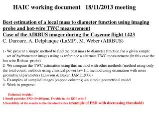
HAIC working document 18/11/2013 meeting. Best estimation of a local mass to diameter function using imaging probe and hot-wire TWC measurement Case of the AIRBUS imager during the Cayenne flight 1423 C. Duroure, A. Delplanque (LaMP), M. Weber (AIRBUS)

E N D
HAIC working document 18/11/2013 meeting Best estimation of a local mass to diameter function using imaging probe and hot-wire TWC measurement Case of the AIRBUS imager during the Cayenne flight 1423 C. Duroure, A. Delplanque (LaMP), M. Weber (AIRBUS) 1- We present a simple method to find the best mass to diameter function for a given sample set of hydrometeor images using as reference a alternate TWC measurement (in this case the hot wire Robust probe) 2- We compare the TWC estimation using this method with other methods (method using only the total count, methods using classical power law fit, method using estimation with more geometrical parameters (Lawson & Baker, JAMC,2006) 3- Examples of sampled images (capped columns) => simple geometrical model 4- Work in progress: Technical trouble: 1-Small particles PSD (D<100µm). Trouble in the ROI code ? 2-Sensibility of the results to the threshold rules (example of PSD with decreasing threshold)
TWC hot wire (Robust) 1 B Best A.M estimate 2 Lawson & B. estimate 3 Ctot estimate Three exemples of TWC estimations from imager using different rules, compared to hot wire probe.
Comparisons between imager and hot wire probe 1 2 3 Scatter plot (TWC from imager, TWC from hot wire probe) 1- Best estimation using power law functions (see next slides) 2- Lawson and Baker geometrical estimation f(A,W,L,P) (non linearity, due to Lmax estimation ?) 3- Simplest estimation (using total count of hydrometeor images)
Estimation of the mass(diameter) function mass=A*Diam^B Sigma using only total concentration Best estimation using PSD and M(D) power law Beta=1.93 B=1.50 B=1.93 B=2.50 1- Look for the best linear correlation of TWC from imager and hot wire (not sensible to theA prefactor, i.e. calibration factors, DOF,….) => Estimation of B
- Imager … Hot wire • Step 2- Look for the best PDF correlation between the two probes • Empirical estimation of the prefactor M= 3.28e-5 Dsur Step 3- Verify the estimated mass to diameter law (Mass=A.DB) assuming: shape model and hydrometeor density 1.93
Capped columns Leg [12 h,12.7 h] Best estimate of B=1.93 Irregular+agregates Leg [12.7 h,12.8 h] Best estimate of B=1.98 (more dense objects ?)
Some examples of « well oriented » images of capped columns (more than 300 avaiable (D> 300µm) for the 10.6 Km leg [12h,12.7h] Manual estimation of 4 geometrical variables: (Lc,Wc) columns part, (Lp,Wp) plates part 1 mm Wp Assumed growth historie of these CP: 1- Start as column for higth sursatuation S 2- Transition to plate for low S Large variability observed for this transition => Dificult to define a « standard » shape Wc Lp Lc
Some examples of « irregular» images (+aggregates+rosettes) for the 10.6 Km altitude sub-leg [12.7 h,12.8h] (« old » region, low concentration) 1 mm Assumed growth historie of these cristal ? 1- Nucleation of supercooled droplet 2- Vapour diffusion process (low S ?) 2- Agregation On the site: CATROI_V1423all Catalogue of all ROI images of size larger than 300µm (for identification of regions)
Tresholding sensibility analysis Treshold definition: Amp=(max(image)-min(image))/2 Med= min(image)+Amp Tresh=med-S*Amp Binary image= image LE Tresh S=0 S=0.1 S=0.2 GEO ROI files on the site V1423_GEO_S000 S=0 V1423_GEO_S010 S=0.1 --------------- V1423_GEO_S030 S=0.3 S=0.25
Tresholding sensibility analysis Small diameter effect Large diameter effect Diameter measure shift (few pixel) Artefact for tail of large particles S=0 S=0.1 S=0.2 S=0.25 S=0 S=0.1 S=0.2 2 pix S=0.25
AIRBUS PSD __ ROI PSD ? Diameter (µm) Diameter (µm) Technical trouble: 1-Small particles PSD (D<100µm). Trouble in the ROI code ? 2-AIRBUS PSD jump ?