Download
1 / 19
190 likes | 341 Views
LogP and BSP models. LogP model. Common MPP organization: complete machine connected by a network. LogP attempts to capture the characteristics of such organization. PRAM model: shared memory. M. M. M. °°°. P. P. P. network. Deriving LogP model. ° Processing

E N D
LogP model • Common MPP organization: complete machine connected by a network. • LogP attempts to capture the characteristics of such organization. PRAM model: shared memory M M M °°° P P P network
Deriving LogP model ° Processing – powerful microprocessor => P ° Communication + significant latency => L + limited bandwidth => g + significant overhead => o - on both ends • no consensus on topology => should not exploit structure – no consensus on programming model => should not enforce one
LogP P ( processors ) P M P M P M ° ° ° o (overhead) o g (gap) L (latency) Limited Volume Interconnection Network ( L/ g to or from a proc) • Latency in sending a (small) mesage between modules • overhead felt by the processor on sending or receiving msg • gap between successive sends or receives (1/BW) • Processors
Using the model • Two processors send n words to each other: • 2o + L + g(n-1) • Assumes no network contention • Can under-estimate the communication time. o o L o o L g time
Develop efficient broadcast algorithm based on the LogP model • Broadcast a single datum to P-1 processors
Strengths of the LogP model • Simple, 4 parameters • Can easily be used to guide the algorithm development, especially algorithms for communication routines. • This model has been used to analyze many collective communication algorithms.
Weaknesses of the LogP model • Accurate only at the very low level (machine instruction level) • Inaccurate for more practical communication systems with layers of protocols (e.g. TCP/IP) • Many variations. • LogP family models: LogGP, logGPC, pLogP, etc • Making the model more accurate and more complex
BSP (Bulk synchronous Parallel) • The BSP abstract computer is a bridging model for designing parallel algorithms • Something between hardware and programming model. • A BSP computer consists of • A set of processor-memory pairs • A communication network that delivers messages in a point-to-point manner • Mechanism for the efficient barrier synchronization for all or a subset of the processes
BSP programs • BSP programs composed of supersteps • In each superstep consists of three ordered stages: • Computation (up to a certain unit) • Communication • Barrier synchronization
BSP programs • Vertical structure • A sequence of supersteps • Local computation • Communication • Barrier synchronization • Horizonal structure • Concurrency among a fixed number of virtual processors • Processes do not have a particular order • Locality plays no role • P = number of processors
BSP programming style • Properties • Simple to write programs • Independent of target architecture • Performance of the model is predictable • Considers computation and communication at the level of the entire program and executing computer instead of individual processes • Renounces locality as an optimization issue. • May not be ideal when locality is critical.
BSP communications • BSP considers communication en masse • bound the total time to deliver the whole set of data in a superstep. • h-relation: the maximum number of incoming or outgoing messages per processor • Parameter g measures the permeability of the network to continuous traffic addressed to uniformly random destinations • Defined such that it takes hg time to deliver an h-relation • BSP does not distinguish between sending 1 message of length m, or m messages of length 1. • Both cost mgh
BSP barrier synchronization • The cost has two parts: • Variation in completion time of computation step • The cost of reach globally consistent state in all processors • Cost is captured by parameter l • Lower bound on l is a function of the diameter of the networks
Predictability of the BSP model • A BSP computer is modeled by: • P: number of processors • S: processor computation speed (flops/s), used to calibrate g and l • l: synchronization periodicity; minimal number of time steps between successive synchronization operations • g: the cost of communication so that an h-relation is realized within gh steps. • Cost of a super step (standard cost model) • Cost of a superstep (overlapping cost model)
Cost of a BSP algorithm • The sum of the costs of all S supersteps • Strategies used in writing efficient BSP programs • Balance the computation in each superstep between processes • W is the maximum of all computation times in different processors • Balance the communication between processes • H is the maximum of the fan-in/fan-out of data • Minimize the number of supersteps • Determine the number of barriers in the program
BSP and PRAM • BSP is a generalization of PRAM • Processes in a superstep can have different computation time • Communication and synchronization costs are explicitly taken into consideration • PRAM does not result in a programming model while BSP has some implementations.
BSP and LogP • Communication in LogP has a “local” view, based on per pair performance, communication in BSP has a “global” view, based on the performance for the whole program • LogP has a term (o) for the communication overhead. • LogP + barriers – overhead = BSP • Both models can efficiently simulate the other.
PRAM, BSP, LogP summary • All are fairly simple and can be used to guide parallel algorithm development. • Simplicity is necessary to be useful for guiding algorithm development, but results in inaccuracy for performance modeling. • Many extensions have proposed to refine the models: trade simplicity for accuracy.