Download
1 / 28
290 likes | 490 Views
RAM, PRAM, and LogP models. Why models?. What is a machine model? An abstraction that describes the operation of a machine Associates a value (cost) with each machine operation Why do we need models? Makes it easier to analyze and develop algorithms

E N D
Why models? • What is a machine model? • An abstraction that describes the operation of a machine • Associates a value (cost) with each machine operation • Why do we need models? • Makes it easier to analyze and develop algorithms • Hides the machine implementation details so that general results that apply to a broad class of machines are obtainable • Analyzes the achievable complexity (time, space, etc.) bounds • Analyzes maximum parallelism • Conversely, models are directly related to algorithms.
RAM (random access machine) model • Memory consists of infinite array (memory cells). • Instructions executed sequentially, one at a time • All instructions take unit time: • Load/store • Arithmetic • Logic • Running time of an algorithm: the number of instructions executed • Memory requirement: the number of memory cells used in the algorithm
RAM (random access machine) model • The RAM model is the base of algorithm analysis for sequential algorithms although it is not perfect: • Memory is not infinite • Not all memory accesses take the same time • Not all arithmetic operations take the same time • Instruction pipelining is not taken into consideration • The RAM model (with asymptotic analysis) often gives relatively realistic results
PRAM (Parallel RAM) • A unbounded collection of processors • Each process has an infinite number of registers • A unbounded collection of shared memory cells • All processors can access all memory cells in unit time (when there is no memory conflict) • All processors execute PRAM instructions synchronously (some processors may be idle) • Each PRAM instruction executes in a 3-phase cycle: • Read from a share memory cell (if needed) • Computation • Write to a share memory cell (if needed)
PRAM (Parallel RAM) • The only way processors exchange data is through the shared memory. Parallel time complexity: the number of synchronous steps in the algorithm Space complexity: the number of shared memory Parallelism: the number of processors used
PRAM All processors can do things in a synchronous manner (with infinite shared memory and infinite local memory). How many steps does it take to complete a task?
PRAM – further refinement • PRAMs are further classifed based on how the memory conflicts are resolved. • Read • Exclusive Read (ER) – all processors can only simultaneously read from distinct memory locations (but not the same location). • What if two processors want to read from the same location? • Concurrent Read (CR) – all processors can simultaneously read from all memory locations.
PRAM – further refinement • PRAMs are further classified based on how the memory conflicts are resolved. • Write • Exclusive Write (EW) – all processors can only simultaneously write to distinct memory locations (but not the same location) • Concurrent Write (CR) – all processors can simultaneously write to all memory locations: • Common CW: only allow the same value to be written to the same location simultaneously • Random CW: randomly pick a value • Priority CW: processors have priority, the value in the highest priority processor wins
PRAM model variations • EREW, CREW, CRCW (common), CRCW (random), CRCW (Priority) • Which model is closer to actual SMP machines? • Model A is computationally stronger than model B if and only if any algorithm written in B will run unchanged in A. We can prove, • EREW <= CREW <= CRCW (common) <= CRCW (random)
PRAM algorithm example • SUM: Add N numbers in memory M[0, 1, …, N-1] • Sequential SUM algorithm (O(N) complexity) for (i=0; i<N; i++) sum = sum + M[i]; • PRAM SUM algorithm?
PRAM SUM algorithm • Which mo Which PRAM model?
PRAM SUM algorithm complexity • Time complexity? • Number of processors needed? • Speedup (vs. sequential program)?
Parallel search algorithm • P processors PRAM with unsorted N numbers (P<=N) • Does x exist in the N numbers? • p_0 has x initially, p_0 must know the answer at the end.
Parallel search algorithm • PRAM Algorithm: • Step 1: Inform everyone what x is • Step 2: every processor checks N/P numbers and sets a flag • Step 3: Check if any flag is set to 1. • EREW: O(log(p)) step 1, O(N/P) step 2, and O(log(p)) step 3. • CREW: O(1) step 1, O(N/P) step 2, and O(log(p)) step 3. • CRCW (common): O(1) step 1, O(N/P) step 2, and O(1) step 3.
PRAM strengths • Natural extension of RAM • It is simple and easy to understand • Communication and synchronization issues are hidden • Can be used as benchmarks • If an algorithm performs badly in the PRAM model, it will perform badly on real machines • A good PRAM program may not be practical, however • It is useful in analyzing threaded algorithms for SMP/multicore machines
PRAM weaknesses • Model inaccuracies • Unbounded local memory (register) • All operations take unit time • Processors run in lock steps • Unaccounted costs • Non-local memory access • Latency • Bandwidth • Memory access contention
PRAM variations • Bounded memory PRAM, PRAM(m) • In a given step, only m memory accesses can be serviced • Bounded number of processors PRAM • Any problem that can be solved by a p processor PRAM in t steps can be solved by a p’ processor PRAM in t = O(tp/p’) steps • LPRAM • L units to access global memory • Any algorithm that runs in a p processor PRAM can run in LPRAM with a loss of a factor of L • BPRAM • L units for the first message • B units for subsequent messages
PRAM summary • The RAM model is widely used • PRAM is simple and easy to understand • This model rarely reaches beyond the algorithm community. • It is getting more important as threaded programming becomes more popular. • The BSP (bulk synchronous parallel) model is another try after PRAM • Asynchronously progress • Model latency and limited bandwidth
LogP model • Common MPP organization: complete machine connected by a network • LogP attempts to capture the characteristics of such organization PRAM model: shared memory M M M °°° P P P network
Deriving LogP model ° Processing – powerful microprocessor, large DRAM, cache => P ° Communication + significant latency => L + limited bandwidth => g + significant overhead => o - on both ends – no consensus on topology => should not exploit structure + limited capacity – no consensus on programming model => should not enforce one
LogP P ( processors ) P M P M P M ° ° ° o (overhead) o g (gap) L (latency) Limited Volume Interconnection Network ( L/ g to or from a proc) • Latency in sending a (small) mesage between modules • overhead felt by the processor on sending or receiving msg • gap between successive sends or receives (1/BW) • Processors
Using the model o o L o o L g time ° Send n messages from proc to proc in time 2o + L + g(n-1) – each processor does o n cycles of overhead – has (g-o)(n-1) + L available compute cycles ° Send n messages from one to many in same time ° Send n messages from many to one in same time – all but L/g processors block so fewer available cycles P P
Using the model • Two processors send n words to each other: • 2o + L + g(n-1) • Assumes no network contention • Can underestimate the communication time
LogP philosophy • Think about: • – mapping of a task onto P processors • – computation within a processor, its cost, and balance • – communication between processors, its cost, and balance • You are given a characterization of processor and network performance • Do not think about what happens within the network
Develop optimal broadcast algorithm based on the LogP model • Broadcast a single datum to P-1 processors
Strengths of the LogP model • Simple, 4 parameters • Can easily be used to guide the algorithm development, especially for algorithms for communication between processors • This model has been used to analyze many collective communication algorithms.
Weaknesses of the LogP model • Accurate only at the very low level (machine instruction level) • Inaccurate for more practical communication systems with layers of protocols (e.g., TCP/IP) • Many variations • LogP family models: LogGP, logGPC, pLogP, etc. • Making the model more accurate and more complex