Enhancing Portable Algorithms and Communication Efficiency in Networked Processing Systems
This paper discusses the limitations of the Bulk Synchronous Parallel (BSP) model in terms of bandwidth and processing element (PE) load, emphasizing the need for improved models that facilitate efficient algorithm execution independent of network topology. It explores innovative communication strategies for optimized message handling and introduces recursive approaches for aggregating computation results, particularly applying Fast Fourier Transform (FFT) on butterfly networks. Additionally, we investigate various data placement strategies and communication schedules to reduce bottlenecks and enhance processing performance across distributed systems.

Enhancing Portable Algorithms and Communication Efficiency in Networked Processing Systems
E N D
Presentation Transcript
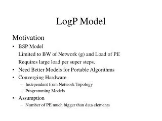
LogP Model Motivation • BSP Model Limited to BW of Network (g) and Load of PE Requires large load per super steps. • Need Better Models for Portable Algorithms • Converging Hardware • Independent from Network Topology • Programming Models • Assumption • Number of PE much bigger than data elements
Parameters • L: Latency • delay on the network • o: Overhead on PE • g: gap • minimum interval between consecutive messages (due to bandwidth) • P: Number of PEs Note: L,o,g : independent from P or node distances Message length: short message L,o,g are per word or per message of fixed length k word message: k short messages (k*o overhead) L independent from message length
Parameters (continue) • Bandwidth: 1/g * unit message length • Number of messages to send or receive for each PE: L/g • Send to Receive total time : L+2o • if o >> g, ignore o • Similar to BSP except no synchronization step • No communication computation overlapping • Speed-up factor at most two
P0 P5 P2 P6 P7 g p0 o L p1 Broadcast Optimal Broad cast tree 0 P1 P3 P4 10 14 18 22 20 24 24 P=8, L=6, g=4, o=2
Optimal Sum • Given time T, how many items we can add? • Approach: recursive • At root, if T <= L+2o use a single PE (can add T+1 items) • If T > L+2o, • Root should have data ready at T, • and sender must have sum ready at T - L - 2o - 1 • Recursively construct the sum tree at the sender • If T - g > L+2o, Root also can receive data, and compute the sum with T-g as the root.
Applications FFT on the Butterfly network • Data Placement • cyclic layout - First log n/P local comm, last log P global • blocked layout - First log P global comm, remaining local • hybrid: After log (n/P) iteration, re-map to cyclic so that remaining can be also local Communication time: g* (n/P**2) (P-1) + L each PE has n/P data, each of 1/P goes to each other PE Total time is (1+g/logn) optimal • All to all Communication schedule • Approach 1: each PE sends PE1, PE2, … => bottle neck at PE1, PE2 in this order • Approach 2 (staggered re-map) -- no congestion • PE1 sends PE2, PE3,.. • PE2 sends PE3, PE4, etc
Implementation on CM5 • CM: • 33MHz • Fat Trees • Global Control for scan/prefix/broadcast • one CM-5 3.2 MFLOPs • FFT on local: 2.8 - 2.2 MFLOPs (cache effect) • each cycle: • multiply and add : 4.5 us • o: 2us • L: 6us • g: 4us • load ans store overhaed per cycle 1us • communication time : n/P max (1us + 2o, g) + L • bottleneck: processing and overhead, not bw
LU decomposition • Data arrangement critical
Matching machine with real machines Average Distance topology independent usually works for n=1024 nodes. The difference between average distance and max distance are not such different
Potential Concerns • Algorithmic concern • Theory? • Too complex? • Communication concerns • how to use trivial comm such as local exchange • topology dependencies?
Comparison with BSP • Length of superstep • message not usable till next step • special hardware for sync • virtual/physical large, context switching may be expensive