Modeling the Effect of Dissolution Temperature on Yield Using JMP
This tutorial demonstrates how to use JMP software to analyze the impact of dissolution temperatures on yield. By utilizing the "Fit Model" capability, we create a mathematical regression model to understand the relationship between temperature (as the factor) and yield (as the response). Steps include inserting yield and temperature data, selecting variables for analysis in the Fit Model window, and generating plots to visualize the results. The session provides a comprehensive summary of fit, ANOVA, and parameter estimates to interpret the model effectively.

Modeling the Effect of Dissolution Temperature on Yield Using JMP
E N D
Presentation Transcript
JMP Example 5 Use the previous yield data from different dissolution temperatures. Make a model that describes the effect of temperature on the yield. Note that here, temperature is the factor and the yield is the response.
Use the “Fit Model” capability to apply to the data. This will help generate a mathematical model around the data supplied.
The “Fit Model” window will appear. The response is always placed in the “Pick Role Variables Y” box, and regression variables are always added to the “Construct Model Effects” Box. Then JMP interprets the data to create the most accurate regression model possible.
Since yield is the response, select yield, and add it to the Y “Pick Role Variables” window.
Since temperature is the only regressor variable, select it and add it to the “Construct Model Effects Window”.
When all factors are added to the “Construct Model Effects” window, run the model.
JMP will automatically generate plots with the “Summary of Fit” data below them.
When you scroll down in the “Fit Least Squares” Window, the model data will be available. This data includes the “Summary of Fit”, “Analysis Of Variance” (a.k.a. ANOVA), and “Parameter Estimates”. Note: the “Parameter Estimates” section gives the regression coefficients.