Modern Control Systems (MCS)
Modern Control Systems (MCS). Lecture-32-33-34 Design of Control Systems in Sate Space Observer Based Approach. Dr. Imtiaz Hussain email: imtiaz.hussain@faculty.muet.edu.pk URL : http://imtiazhussainkalwar.weebly.com/. Lecture Outline. Introduction State Observer


Modern Control Systems (MCS)
E N D
Presentation Transcript
Modern Control Systems (MCS) Lecture-32-33-34 Design of Control Systems in Sate Space Observer Based Approach Dr. Imtiaz Hussain email: imtiaz.hussain@faculty.muet.edu.pk URL :http://imtiazhussainkalwar.weebly.com/
Lecture Outline • Introduction • State Observer • Topology of Pole Placement (Observer based) • Full Order State Observer • Reduced Order state Observer • Using Transformation Matrix P • Direct Substitution Method • Ackermann’s Formula
Introduction • In the pole-placement approach to the design of control systems, we assumed that all state variables are available for feedback. • In practice, however, not all state variables are available for feedback. • Then we need to estimate unavailable state variables.
Introduction • Estimation of unmeasurable state variables is commonly called observation. • A device (or a computer program) that estimates or observes the state variables is called a state estimator, state observer, or simply an observer. • There are two types of state observers • Full Order State Observer • If the state observer observes all state variables of the system, regardless of whether some state variables are available for direct measurement, it is called a full-order state observer. • Reduced Order State Observer • If the state observer observes only those state variables which are not available for direct measurement, it is called a reduced-order state observer.
Topology of State Feedback Control with Observer Based Approach • State feedback with state observer
Topology of State Feedback Control with Observer Based Approach • State feedback Control
Topology of State Feedback Control with Observer Based Approach • State Feedback with observer
State Observer • A state observer estimates the state variables based on the measurements of the output and control variables. • Here the concept of observability plays an important role. • State observers can be designed if and only if the observability condition is satisfied.
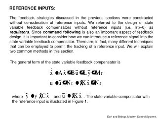
State Observer • Consider the plant defined by • The mathematical model of the observer is basically the same as that of the plant, except that we include an additional term that includes the estimation error to compensate for inaccuracies in matrices A and B and the lack of the initial error. • The estimation error or observation error is the difference between the measured output and the estimated output. • The initial error is the difference between the initial state and the initial estimated state.
State Observer • Thus we define the mathematical model of observer to be • Where is estimated state vector, is estimated output and is observer gain matrix.
Full Order State Observer • The order of the state observer that will be discussed here is the same as that of the plant. • Consider the plant define by following equations • Equation of state observer is given as • To obtain the observer error equation, let us subtract Equation (2) from Equation (1): (1) (2)
Full Order State Observer • Simplifications in above equation yields • Define the difference between and as the error vector e. • Equation (3) can now be written as (3)
Full Order State Observer • From above we see that the dynamic behavior of the error vector is determined by the eigenvalues of matrix A-KeC. • If matrix A-KeCis a stable matrix, the error vector will converge to zero for any initial error vector e(0). • That is, will converge to regardless of the values of x(0). • And if the eigenvalues of matrix A-KeCare chosen in such a way that the dynamic behavior of the error vector is asymptotically stable and is adequately fast, then any error vector will tend to zero (the origin) with an adequate speed.
Full Order State Observer • If the plant is completely observable, then it can be proved that it is possible to choose matrix Ke such that A-KeChas arbitrarily desired eigenvalues. • That is, the observer gain matrix Ke can be determined to yield the desired matrix A-KeC.
Duality Property • The design of the full-order observer becomes that of determining an appropriate Ke such that A-KeChas desired eigenvalues. • Thus, the problem here becomes the same as the pole-placement problem. • In fact, the two problems are mathematically the same. • This property is called duality.
Duality Property • Consider the system defined by • In designing the full-order state observer, we may solve the dual problem, that is, solve the pole-placement problem for the dual system. • Assuming the control signal to be
Duality Property • If the dual system is completely state controllable, then the state feedback gain matrix Kcan be determined such that matrix A*-C*K will yield a set of the desired eigenvalues. • If , ,…, , are the desired eigenvalues of the state observer matrix, then by taking the same as the desired eigenvalues of the state-feedback gain matrix of the dual system, we obtain • Noting that the eigenvalues of A*-C*K and those of A-K*Care the same, we have
Duality Property • Comparing the characteristic polynomial and the characteristic polynomial for the observer system , we find that Ke and K* are related by • Thus, using the matrix Kdetermined by the pole-placement approach in the dual system, the observer gain matrix Ke for the original system can be determined by using the relationship Ke=K*.
Observer Gain Matrix • Using Transformation Matrix Q • Direct Substitution Method • Ackermann’s Formula
Observer Gain Matrix • Using Transformation Matrix Q • Since
Observer Gain Matrix • Direct Substitution Method
Observer Gain Matrix • Ackermann’s Formula • For the dual system • Since
Observer Gain Matrix • Simplifying it further
Observer Gain Matrix • The feedback signal through the observer gain matrix Ke serves as a correction signal to the plant model to account for the unknowns in the plant. • If significant unknowns are involved, the feedback signal through the matrix Ke should be relatively large. • However, if the output signal is contaminated significantly by disturbances and measurement noises, then the output y is not reliable and the feedback signal through the matrix Ke should be relatively small.
Observer Gain Matrix • The observer gain matrix Ke depends on the desired characteristic equation • The observer poles must be two to five times faster than the controller poles to make sure the observation error (estimation error) converges to zero quickly. • This means that the observer estimation error decays two to five times faster than does the state vector x. • Such faster decay of the observer error compared with the desired dynamics makes the controller poles dominate the system response.
Observer Gain Matrix • It is important to note that if sensor noise is considerable, we may choose the observer poles to be slower than two times the controller poles, so that the bandwidth of the system will become lower and smooth the noise. • In this case the system response will be strongly influenced by the observer poles. • If the observer poles are located to the right of the controller poles in the left-half s plane, the system response will be dominated by the observer poles rather than by the control poles.
Observer Gain Matrix • In the design of the state observer, it is desirable to determine several observer gain matrices Ke based on several different desired characteristic equations. • For each of the several different matrices Ke , simulation tests must be run to evaluate the resulting system performance. • Then we select the best Ke from the viewpoint of overall system performance. • In many practical cases, the selection of the best matrix Ke boils down to a compromise between speedy response and sensitivity to disturbances and noises.
Example-1 • Consider the system • We use observer based approach to design state feedback control such that • Design a full-order state observer assume that the desired eigenvalues of the observer matrix are , .
Example-1 • Let us examine the observability matrix first • Since rank(OM)=2 the given system is completely state observable and the determination of the desired observer gain matrix is possible.
Example-1 (Method-1) • The given system is already in the observable canonical form. Hence, the transformation matrix Qis I.
Example-1 (Method-1) • The characteristic equation of the given system is • We have
Example-1 (Method-1) • The desired characteristic equation of the system is • We have
Example-1 (Method-1) • Observer gain matrix Ke can be calculated using following formula • Where
Example-1 (Method-2) • The characteristic equation of observer error matric is • Assuming
Example-1 (Method-2) • The desired characteristic polynomial is • Comparing coefficients of different powers of s
Example-1 (Method-3) • Using Ackermann’s formula • Where
Example-1 (Method-3) • Using Ackermann’s formula
Example-1 • We get the same Ke regardless of the method employed. • The equation for the full-order state observer is given by
Example-2 • Design a regulator system for the following plant: • The desired closed-loop poles for this system are at , . Compute the state feedback gain matrix K to place the poles of the system at desired location. • Suppose that we use the observed-state feedback control instead of the actual-state feedback. The desired eigenvalues of the observer matrix are , . • Obtain the observer gain matrix Ke and draw a block diagram for the observed-state feedback control system.
To download this lecture visit http://imtiazhussainkalwar.weebly.com/ End of Lectures-32-33-34