Download

1 / 38
490 likes | 1.4k Views
Modern Control Systems (MCS). Lecture-27-28 Stability of Digital Control Systems. Dr. Imtiaz Hussain Assistant Professor email: imtiaz.hussain@faculty.muet.edu.pk URL : http://imtiazhussainkalwar.weebly.com/. Lecture Outline. Introduction Asymptotic Stability BIBO Stability

E N D
Modern Control Systems (MCS) Lecture-27-28 Stability of Digital Control Systems Dr. Imtiaz Hussain Assistant Professor email: imtiaz.hussain@faculty.muet.edu.pk URL :http://imtiazhussainkalwar.weebly.com/
Lecture Outline • Introduction • Asymptotic Stability • BIBO Stability • Internal Stability • Routh Hurwitz Stability Criterion for DT Systems • Jury’s Stability Test
Introduction • Stability is a basic requirement for digital and analog control systems. • Digital control is based on samples and is updated every sampling period, and there is a possibility that the system will become unstable between updates. This obviously makes stability analysis different in the digital case. • There are different definitions and tests of the stability of linear time-invariant (LTI) digital systems based on transfer function models. • Input-output stability and internal stability. • Routh-Hurwitz criterion • Jury criterion, and the Nyquist criterion. • Gain margin and phase margin for digital systems
Asymptotic Stability • The most commonly used definitions of stability are based on the magnitude of the system response in the steady state. If the steady-state response is unbounded, the system is said to be unstable. • Asymptotic Stability: A system is said to be asymptotically stable if its response to any initial conditions decays to zero asymptotically in the steady state. • If the response due to the initial conditions remains bounded but does not decay to zero, the system is said to be marginally stable.
Asymptotic Stability • In the absence of pole-zero cancellation, an LTI digital system is asymptotically stable if its transfer function poles are in the open unit disc and marginally stable if the poles are in the closed unit disc with no repeated poles on the unit circle. • The open unit disc is the region in the complex plane defined by • The closed unit disc is the region in the complex plane defined by Unit Disc: Adisc with radius 1.
Asymptotic Stability where • Consider a LTI system governed by difference equation • With initial conditions . • Using the z-transform of the output the response of the system due to the initial conditions with the input zero is of the form • where N(z) is a polynomial dependent on the initial conditions.
Asymptotic Stability • Because transfer function zeros arise from transforming the input terms, they have no influence on the response due to the initial conditions. • The denominator of the output z-transform is the same as the denominator of the z-transfer function in the absence of pole-zero cancellation. • Hence, the poles of the function Y(z) are the poles of the system transfer function. • Thus, the output due to the initial conditions is bounded for system poles in the closed unit disc with no repeated poles on the unit circle. It decays exponentially for system poles in the open unit disc (i.e., inside the unit circle).
Example-1 • Determine the asymptotic stability of the following systems:
BIBO Stability • The second definition of stability concerns the forced response of the system for a bounded input. • A bounded input satisfies the condition • A bounded sequence satisfying the constraint |u(k)| < 3 is shown in the figure. Bounded sequence with bound bu= 3
BIBOStability • Bounded-Input–Bounded-Output Stability. A system is said to be bounded-input–bounded-output (BIBO) stable if its response to any bounded input remains bounded. • That is, for any input satisfying • The output satisfies
BIBO Stability • BIBO stability concerns the response of a system to a bounded input. • The response of the system to any input is given by the convolution summation • Where is impulse response sequence.
Asymptotic vs. BIBO Stability • LTI systems, with no pole-zero cancellation, BIBO and asymptotic stability are equivalent and can be investigated using the same tests. • Hence, the term stability is used in the sequel to denote either BIBO or asymptotic stability with the assumption of no unstable pole-zero cancellation.
Internal Stability • So far, we have only considered stability as applied to an open-loop system. • However, the stability of the closed-loop transfer function is not always sufficient for proper system operation because some of the internal variables may be unbounded. • In a feedback control system, it is essential that all the signals in the loop be bounded when bounded exogenous inputs are applied to the system.
Internal Stability • Consider a unity feedback digital control system shown in following figure. The system has two outputs, Y and U, and two inputs, R and D. • The transfer functions associated with the system are given by
Internal Stability • If all the transfer functions that relate system inputs (R and D) to the possible system outputs (Y and U) are BIBO stable, then the system is said to be internally stable.
Routh-Hurwitz Criterion • The Routh-Hurwitz criterion determines conditions for left half plane (LHP) polynomial roots and cannot be directly used to investigate the stability of discrete-time systems. • The bilinear transformation transforms the inside of the unit circle to the LHP. This allows the use of the Routh-Hurwitz criterion for the investigation of discrete-time system stability. • The bilinear Transformation is a special case of conformal mapping used to convert continuous LTI transfer function into discrete shift invariant transfer function.
Routh-Hurwitz Criterion • For the general z-polynomial, • Using the bilinear transformation • The Routh-Hurwitz approach becomes progressively more difficult as the order of the z-polynomial increases. But for low-order polynomials, it easily gives stability conditions.
Example-2 • By using Routh-Hurwitz stability criterion, determine the stability of the following digital systems whose characteristic are given as. • Transforming the characteristic equationinto by using the bilinear transformation gives: Solution
Example-2 • Routh array can now be developed from the transformed characteristic equation. • Since there are no sign changes in the first column of the Routh array therefore the system is stable.
Example-3 • By using Routh-Hurwitz stability criterion, determine the stability of the following digital systems whose characteristic are given as. • Transforming the characteristic equation into by using the bilinear transformation gives: Solution
Example-3 • Routh array can now be developed from the transformed characteristic equation. • From the table above, since there is one sign change in the first column above equation has one root in the right-half of the w-plane. • This, in turn, implies that there will be one root of the characteristic equation outside of the unit circle in the z-plane.
Jury’s Stability Test • Stability test method presented by Eliahu Ibraham Jury. • It is possible to investigate the stability of z-domain polynomials directly using the Jury test. • These tests involve determinant evaluations as in the Routh-Hurwitz test for s-domain polynomials but are more time consuming.
Jury’s Stability Test • For a polynomial • the roots of the polynomial are inside the unit circle if and only if
Jury’s Stability Test • Where the terms in the n+1 conditions are calculated from following Table.
Jury’s Stability Test • The entries of the table are calculated as follows
Example-4 • Test the stability of the polynomial. • Develop Jury’s Table [(2n-3) rows]. Solution
Example-4 • 3rd row is calculated using
Example-4 • 4rth row is same as 3rd row in reverse order
Example-4 • 5th row is calculated using
Example-4 • 6th row is same as 5th row in reverse order
Example-4 • 7th row is calculated using
Example-4 • Now we need to evaluate following conditions nth order system 5th order System
Example-4 • The first two conditions require the evaluation of F(z) at z = ±1. Satisfied Not Satisfied
Example-4 • Next four conditions require Jury’s table Satisfied Not Satisfied Satisfied Satisfied
Example-5 • Test the stability of the polynomial. • Develop Jury’s Table [(2n-3) rows]. Solution Satisfied Satisfied
Example-5 • Next four conditions require Jury’s table • Since all the conditions are satisfied, the system is stable. Satisfied
Example-6 • Determine the stability of a discrete data system described by the following CE by using Jury’s Stability criterion.
To download this lecture visit http://imtiazhussainkalwar.weebly.com/ End of Lectures-27-28