Modern Control Systems (MCS)
Modern Control Systems (MCS). Lecture-16-17-18 Lag Compensation. Dr. Imtiaz Hussain Assistant Professor email: imtiaz.hussain@faculty.muet.edu.pk URL : http://imtiazhussainkalwar.weebly.com/. Lecture Outline. Introduction to lag compensation Electronic Lag Compensator

Modern Control Systems (MCS)
E N D
Presentation Transcript
Modern Control Systems (MCS) Lecture-16-17-18 Lag Compensation Dr. Imtiaz Hussain Assistant Professor email: imtiaz.hussain@faculty.muet.edu.pk URL :http://imtiazhussainkalwar.weebly.com/
Lecture Outline • Introduction to lag compensation • Electronic Lag Compensator • Mechanical Lag Compensator • Electrical Lag Compensator • Design Procedure of Lag Compensator • Examples
Lag Compensation • Lag compensation is used to improve the steady state error of the system. • Generally Lag compensators are represented by following transfer function • Or • Where is gain of lag compensator. , () , ()
Lag Compensation , ()
Lag Compensation • Consider the problem of finding a suitable compensation network for the case where the system exhibits satisfactory transient-response characteristics but unsatisfactory steady-state characteristics. • Compensation in this case essentially consists of increasing the open loop gain without appreciably changing the transient-response characteristics. • This means that the root locus in the neighborhood of the dominant closed-loop poles should not be changed appreciably, but the open-loop gain should be increased as much as needed.
Lag Compensation • To avoid an appreciable change in the root loci, the angle contribution of the lag network should be limited to a small amount, say less than 5°. • To assure this, we place the pole and zero of the lag network relatively close together and near the origin of the s plane. • Then the closed-loop poles of the compensated system will be shifted only slightly from their original locations. Hence, the transient-response characteristics will be changed only slightly.
Lag Compensation , () • Consider a lag compensator Gc(s), where • If we place the zero and pole of the lag compensator very close to each other, then at s=s1 (where s1is one of the dominant closed loop poles then the magnitudes and are almost equal, or
Lag Compensation • To make the angle contribution of the lag portion of the compensator small, we require • This implies that if gain of the lag compensator is set equal to 1, the alteration in the transient-response characteristics will be very small, despite the fact that the overall gain of the open-loop transfer function is increased by a factor of , where >1.
Lag Compensation • If the pole and zero are placed very close to the origin, then the value of can be made large. • A large value of may be used, provided physical realization of the lag compensator is possible. • It is noted that the value of T must be large, but its exact value is not critical. • However, it should not be too large in order to avoid difficulties in realizing the phase-lag compensator by physical components.
Lag Compensation • An increase in the gain means an increase in the static error constants. • If the open loop transfer function of the uncompensated system is G(s), then the static velocity error constant Kv of the uncompensated system is • Then for the compensated system with the open-loop transfer function Gc(s)G(s) the static velocity error constant becomes
Lag Compensation • The main negative effect of the lag compensation is that the compensator zero that will be generated near the origin creates a closed-loop pole near the origin. • This closed loop pole and compensator zero will generate a long tail of small amplitude in the step response, thus increasing the settling time.
Electronic Lag Compensator • The configuration of the electronic lag compensator using operational amplifiers is the same as that for the lead compensator.
Electronic Lag Compensator • Pole-zero Configuration of Lag Compensator
Electrical Lag Compensator • Following figure shows lag compensator realized by electrical network.
Electrical Lag Compensator • Then the transfer function becomes
Electrical Lag Compensator • If an RC circuit is used as a lag compensator, then it is usually necessary to add an amplifier with an adjustable gain so that the transfer function of compensator is
Design Procedure • The procedure for designing lag compensators by the root-locus method may be stated as follows. • We will assume that the uncompensated system meets the transient-response specifications by simple gain adjustment. • If this is not the case then we need to design a lag-lead compensator which we will discuss in next few classes.
Design Procedure • Step-1 • Draw the root-locus plot for the uncompensated system whose open-loop transfer function is G(s). • Based on the transient-response specifications, locate the dominant closed-loop poles on the root locus.
Design Procedure • Step-2 • Assume the transfer function of the lag compensator to be given by following equation • Then the open-loop transfer function of the compensated system becomes Gc(s)G(s). =
Design Procedure • Step-3 • Evaluate the particular static error constant specified in the problem. • Determine the amount of increase in the static error constant necessary to satisfy the specifications.
Design Procedure • Step-4 • Determine the pole and zero of the lag compensator that produce the necessary increase in the particular static error constant without appreciably altering the original root loci. • The ratio of the value of gain required in the specifications and the gain found in the uncompensated system is the required ratio between the distance of the zero from the origin and that of the pole from the origin.
Design Procedure • Step-5 • Draw a new root-locus plot for the compensated system. • Locate the desired dominant closed-loop poles on the root locus. • (If the angle contribution of the lag network is very small—that is, a few degrees—then the original and new root loci are almost identical. • Otherwise, there will be a slight discrepancy between them. • Then locate, on the new root locus, the desired dominant closed-loop poles based on the transient-response specifications.
Design Procedure • Step-6 • Adjust gain of the compensator from the magnitude condition so that the dominant closed-loop poles lie at the desired location. • will be approximately 1.
Example-1 • Consider the system shown in following figure. • The damping ratio of the dominant closed-loop poles is . The undamped natural frequency of the dominant closed-loop poles is 0.673 rad/sec. The static velocity error constant is 0.53 sec–1. • It is desired to increase the static velocity error constant Kv to about 5 sec–1without appreciably changing the location of the dominant closed-loop poles.
Example-1 (Step-1) • The dominant closed-loop poles of given system are s = -0.3307 ± j0.5864
Example-1 (Step-2) • According to given conditions we need to add following compensator to fulfill the requirement. =
Example-1 (Step-3) • The static velocity error constant of the plant () is • The desired static velocity error constant () of the compensated system is .
Example-1 (Step-4) • Place the pole and zero of the lag compensator • Since , therefore = =
Example-1 (Step-4) Solution-1 • Place the zero and pole of the lag compensator at s=–0.05 and s=–0.005, respectively. • The transfer function of the lag compensator becomes • Open loop transfer function is given as = = =
Example-1 (Step-5) Solution-1 • Root locus of uncompensated and compensated systems. • New Closed Loop poles are
Example-1 (Step-5) Solution-1 • Root locus of uncompensated and compensated systems.
Example-1 (Step-6) Solution-1 • The open-loop gain K is determined from the magnitude condition. • Then the compensator gain is determined as
Example-1 (Step-6) Solution-1 • Then the compensator transfer function is given as
Example-1 (Final Design Check) Solution-1 • The compensated system has following open loop transfer function. • Static velocity error constant is calculated as =
Example-1 (Step-4) Solution-2 • Place the zero and pole of the lag compensator at s=–0.01and s=–0.001, respectively. • The transfer function of the lag compensator becomes • Open loop transfer function is given as = = =
Example-1 (Step-5) Solution-2 • Root locus of uncompensated and compensated systems. • New Closed Loop poles are
Example-2 • Design a lag compensator for following unity feedback system such that the static velocity error constant is 50 sec-1 without appreciably changing the closed loop poles, which are at.
To download this lecture visit http://imtiazhussainkalwar.weebly.com/ End of Lecture-16-17-18