Download
1 / 35
350 likes | 435 Views
Explore the interaction between supermassive black holes and galactic bulges, crucial for galaxy evolution. Presenting numerical model results, movies, and analytical interpretations to shed light on AGN feeding mechanisms. Discuss the missing satellites problem, SMBH growth, and the role of AGN feedback.

E N D
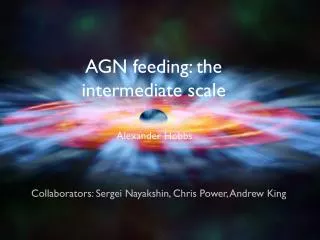
AGN feeding: the intermediate scale Alexander Hobbs Collaborators: Sergei Nayakshin, Chris Power, Andrew King
Talk outline 1) Introduction & motivation 2) Outline of numerical model 3) Results of the model (inc. movies) 4) Analytical interpretation 5) Conclusions
1) Introduction & motivation Baryonic mass function of galaxies (data points) compared to CDM mass spectrum Missing satellites problem! Lines are fits by Hubble type Data from SDSS and Subaru 8m deep wide-angle survey Missing satellites problem - Explained via SNe feedback in shallow potential well AGN feedback? High mass end of spectrum - AGN feedback ??? For AGN feedback need to know how supermassive BHs accrete gas...AGN feeding problem! Figure credit: Read & Trentham 2005
1) Introduction & motivation Supermassive black holes (SMBHs) lurk at centres of galaxies with bulges/spheroids (Kormendy & Richstone 1995) Tight correlation between SMBH properties and bulge properties (Ferrarese & Merritt 2000, Magorrian et al. 1998) Mbh - Mbh - Mbulge Growth of SMBHs closely related to formation of host Co-evolution of SMBHs and galaxy populations requires understanding of how AGN are fed Figure credit: MPA Garching, Volker Springel BHs start out as seeds in early universe (z 14) with masses 103 Msun Observations of high redshift quasars (z 6, 1047 erg s-1) suggest SMBH masses 109 Msun(Kurk et al. 2007) Require BHs to grow close to Eddington limit for 1 Gyr!
1) Introduction & motivation Supermassive black holes (SMBHs) lurk at centres of galaxies with bulges/spheroids (Kormendy & Richstone 1995) Tight correlation between SMBH properties and bulge properties (Ferrarese & Merritt 2000, Magorrian et al. 1998) Mbh - Mbh - Mbulge Growth of SMBHs closely related to formation of host Co-evolution of SMBHs and galaxy populations requires understanding of how AGN are fed Figure credit: MPA Garching, Volker Springel BHs start out as seeds in early universe (z 14) with masses 103 Msun Observations of high redshift quasars (z 6, 1047 erg s-1) suggest SMBH masses 109 Msun(Kurk et al. 2007) Require BHs to grow close to Eddington limit for 1 Gyr!
1) Introduction & motivation Supermassive black holes (SMBHs) lurk at centres of galaxies with bulges/spheroids (Kormendy & Richstone 1995) Tight correlation between SMBH properties and bulge properties (Ferrarese & Merritt 2000, Magorrian et al. 1998) Mbh - Mbh - Mbulge Growth of SMBHs closely related to formation of host Co-evolution of SMBHs and galaxy populations requires understanding of how AGN are fed Figure credit: MPA Garching, Volker Springel BHs start out as seeds in early universe (z 14) with masses 103 Msun Observations of high redshift quasars (z 6, 1047 erg s-1) suggest SMBH masses 109 Msun(Kurk et al. 2007) Require BHs to grow close to Eddington limit for 1 Gyr!
1) Introduction & motivation Supermassive black holes (SMBHs) lurk at centres of galaxies with bulges/spheroids (Kormendy & Richstone 1995) Tight correlation between SMBH properties and bulge properties (Ferrarese & Merritt 2000, Magorrian et al. 1998) Mbh - Mbh - Mbulge Growth of SMBHs closely related to formation of host Co-evolution of SMBHs and galaxy populations requires understanding of how AGN are fed Figure credit: MPA Garching, Volker Springel BHs start out as seeds in early universe (z 14) with masses 103 Msun *poetic license* Observations of high redshift quasars (z 6, 1047 erg s-1) suggest SMBH masses 109 Msun(Kurk et al. 2007) Require BHs to grow close to Eddington limit for 1 Gyr!
Large-scale (hydro + DM) simulations Quarter of a billion gas and dark matter particles Cubic box 100 million light years across 2000 CPUs (Pittsburgh Supercomputing Centre) Gas density increasing with brightness, yellow circles indicate BHs Figure credit: Cornell Theory Center, Princeton Figure credit: Tiziana Di Matteo, Carnegie Mellon University 134 million gas particles, 17 million dark matter particles Projected density of slab 8 Mpc deep Colors show increasing density on logarithmic scale: black (least dense), blue, green, yellow, red, white (most dense)
Large-scale (hydro + DM) simulations Limited computational resources – necessary to use “sub-grid” prescriptions - Feedback (from AGN, supernovae) - SMBH growth Currently treated with Bondi-Hoyle accretion (Bondi 1952) i) Gas has angular momentum! estimate physically wrong ii) Density under-resolved in simulations estimate numerically wrong - arbitrary numerical factors used to enhance accretion rate Need a physically motivated sub-grid prescription for accretion onto an SMBH Require an understanding of the flow on scales of a galactic bulge ( hundreds of pc) - currently under-represented! Need to bridge gap between pc and kpc scales...
2) Numerical model Ran simulations using SPH code GADGET-3 (Springel 2005) • Nsph = 4 x 10⁶ particles • Computational domain 0.1 pc – 100 pc • Adaptive smoothing lengths down to hmin = 2.8 x 10⁻² pc • - Fixed artificial viscosity (Monaghan-Balsara form with = 1) Gravitational forces implemented via background potential (no gas self-gravity) • Central SMBH of Mbh = 108 Msun • Isothermal potential r-2 with scale radius a = 1 kpc, Ma = 1010 Msun • Constant density core within r < 20 pc, Mcore = 2 x 10⁸ Msun Mass enclosed within radius r: One-dimensional velocity dispersion:
2) Numerical model Initial conditions for simulations • Uniform density, spherically-symmetric thick gaseous shell • Mshell = 5.1 x 10⁷ Msun • rin = 30 pc, rout = 100 pc • Cut from relaxed glass-like particle configuration • Isothermal T = 103 K • Accretion (capture) radius racc = 1 pc Velocity field: net rotation + turbulent spectrum Rotation about z-axis with constant v - varying between 0 and 100 km s Turbulence seeded as a Gaussian random field in velocity,with a Kolmogorov spectrum - varying between 0 and 400 km s-1 - divergence-free - max 60 pc
“Laminar” initial conditions Angular momentum conservation and symmetry Formation of geometrically thin disc in xy-plane
“Laminar” initial conditions Majority of gas stays uniform as it falls in Radial shocks in disc plane lead to mixing of gas with different angular momenta
Turbulent initial conditions Turbulent flow creates long dense filaments Flow exhibits strong density contrasts of up to three orders of magnitude
Turbulent initial conditions Some signatures of net rotation retained but far more isotropic than laminar case
3) Results - turbulence and accretion Mass accreted by SMBH strongly correlates with strength of imposed turbulence Accreted mass vs. time for simulations with vrot = 100 km s-1 and varying strengths of vturb. Key: no turbulence (solid black), vturb = 20 km s-1 (black dotted), vturb = 40 km s-1 (black dashed), vturb = 60 km s-1 (black dot-dashed), vturb = 100 km s-1 (brown dot-dot-dash), vturb = 200 km s-1 (red dashed), vturb = 300 km s-1 (pink dotted), vturb = 400 km s-1 (blue dashed)
3) Results - turbulence and accretion Mass accreted by SMBH strongly correlates with strength of imposed turbulence Mass accreted increases rapidly with increasing vturb while vturb << vrot but saturates when vturb vrot Accreted mass vs. time for simulations with vrot = 100 km s-1 and varying strengths of vturb. Key: no turbulence (solid black), vturb = 20 km s-1 (black dotted), vturb = 40 km s-1 (black dashed), vturb = 60 km s-1 (black dot-dashed), vturb = 100 km s-1 (brown dot-dot-dash), vturb = 200 km s-1 (red dashed), vturb = 300 km s-1 (pink dotted), vturb = 400 km s-1 (blue dashed)
3) Results - turbulence and accretion Mass accreted by SMBH strongly correlates with strength of imposed turbulence Mass accreted increases rapidly with increasing vturb while vturb << vrot but saturates when vturb vrot Turbulence broadens angular momentum distribution, putting some gas on low L orbits Accreted mass vs. time for simulations with vrot = 100 km s-1 and varying strengths of vturb. Key: no turbulence (solid black), vturb = 20 km s-1 (black dotted), vturb = 40 km s-1 (black dashed), vturb = 60 km s-1 (black dot-dashed), vturb = 100 km s-1 (brown dot-dot-dash), vturb = 200 km s-1 (red dashed), vturb = 300 km s-1 (pink dotted), vturb = 400 km s-1 (blue dashed) L
Accretion rate trend: i) with rotation Increased net rotation acts to decrease accreted mass in all cases With no turbulence, large decrease in accretion when small amount of angular momentum added High turbulence flattens slope of trend, preventing such a high reduction in accretion Turbulence significantly lessens importance of net rotation in reducing accretion rate For a given (finite) rotation velocity, turbulence enhances accretion Accreted mass by t = 106 yrs vs. rotation velocity for simulations with varying strengths of vturb. Key: no turbulence (solid black), vturb = 20 km s-1 (black dotted), vturb = 40 km s-1 (black dashed), vturb = 60 km s-1 (black dot-dashed), vturb = 100 km s-1 (brown dot-dot-dash), vturb = 200 km s-1 (red dashed), vturb = 300 km s-1 (pink dotted), vturb = 400 km s-1 (blue dashed)
Accretion rate trend: ii) with turbulence Accretion onto SMBH increases significantly with increasing turbulence Trend saturates once vturb > vrot, and begins to slowly decrease as turbulence increased further Weak turbulence -Broadens angular momentum distribution Strong turbulence - Strong density enhancements -Dense regions propagate unaffected by hydrodynamical drag - ‘Ballistic’ motion of high density gas? Accreted mass by t = 106 yrs vs. mean turbulent velocity for runs with varying strengths of vrot. Key: no rotation (solid), vrot = 20 km s-1 (dotted), vrot = 40 km s-1 (dashed), vrot = 60 km s-1 (dot-dashed), vrot = 80 km s-1 (dot-dot-dash), vrot = 100 km s-1 (long dashes) ...loss-cone argument
4) Analytical interpretation: f(v) spectrum vrot Analyse result of this integral in three extremes:
4) Analytical interpretation: f(v) spectrum vrot Analyse result of this integral in three extremes: actual i) when vturb >> vrot
4) Analytical interpretation: f(v) spectrum vrot Analyse result of this integral in three extremes: max i) when vturb vrot
4) Analytical interpretation: f(v) spectrum vrot Analyse result of this integral in three extremes: min i) when vturb << vrot
...agrees with results Trend with size of shell at t = 5 x 10⁵ yrs Error bars t/3 Trend with accretion radius at t = 5 x 10⁵ yrs Error bars t/3 vturb << vrot min vturb >> vrot actual Key: vturb vrot max
...agrees with results Accreted mass trend with rotation velocity
...agrees with results Accreted mass trend with rotation velocity when vturb vrot max
5) Conclusions - In the presence of net rotation, turbulence can enhance accretion (for a given rotation velocity) ...by up to 3-4 orders of magnitude! - For our particular initial condition, runs without turbulence form rings rather than discs ...whereas runs with high turbulence form discs - Accretion trend with turbulence saturates at vturb vrot - Weak turbulence trend broadening of angular momentum distribution - Strong turbulence trend ballistic trajectories of high density gas Key points: -Taken one of the first steps in modelling the intermediate-scale flow in a galactic potential -Identified a possible ‘ballistic’ mode of AGN feeding -If supernovae-driven turbulence can enhance accretion rate onto SMBH then this speaks to a starburst-AGN connection such as is observed (e.g. Farrah et al. 2003)
Future work Take input from cosmological/galactic merger simulations as outer boundary condition Couple accretion model to a physically-motivated feedback prescription (w. Chris Power) embed SMBH feeding and feedback model into large-scale simulation Goal: