Assignment 2 Remarking

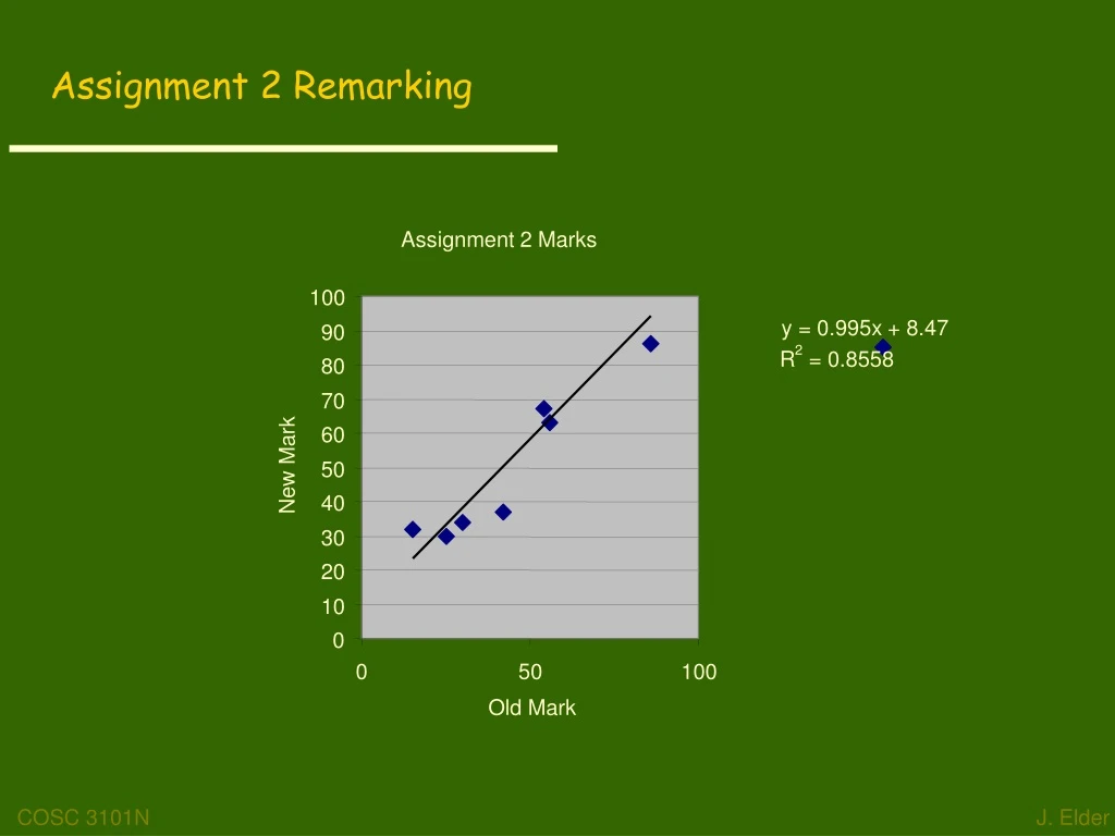
1. y = 0.995x + 8.47 2 R = 0.8558 Assignment 2 Remarking Assignment 2 Marks 100 90 80 70 60 New Mark 50 40 30 20 10 0 0 50 100 Old Mark

2. Section V. Graph Algorithms

3. Idea: send out search ‘wave’ from s. Keep track of progress by colouring vertices: Undiscovered vertices are coloured white Just discovered vertices (on the wavefront) are coloured grey. Previously discovered vertices (behind wavefront) are coloured black. Breadth-First Search

4. Each vertex assigned finite d value at most once. d values assigned are monotonically increasing over time. Q contains vertices with d values {i, …, i, i+1, …, i+1} Time = O(V+E) Breadth-First Search Algorithm

5. Explore every edge, starting from different vertices if necessary. As soon as vertex discovered, explore from it. Keep track of progress by colouring vertices: White: undiscovered vertices Grey: discovered, but not finished (still exploring from it) Black: finished (found everything reachable from it). Depth-First Search

6. Depth-First Search Algorithm

7. Remember: BFS(G,s) finds the shortest paths from a specified vertex s. If G is either undirected and not connected, or directed and not strongly connected, not all vertices of the graph will be visited in BFS. In contrast, DFS(G) visits all vertices, restarting at multiple source vertices if necessary. Why is BFS O(S+V), while DFS is (S+V)?

8. An Application of DFS: Topological Sorting

9. Strongly Connected Components

10. Component Graph

11. Lemma

12. SCC Algorithm

13. Lemma

14. So why does the SCC Algorithm work?

15. Example Problem You are planning a new terrestrial telecommunications network to connect a number of remote mountain villages in a developing country. The cost of building a link between pairs of neighbouring villages (u,v) has been estimated: w(u,v). You seek the minimum cost design that ensures each village is connected to the network. The solution is called a minimum spanning tree. Minimum Spanning Trees

16. Iteratively construct the set of edges A in the MST. Initialize A to {} As we add edges to A, maintain a Loop Invariant: A is a subset of some MST Maintain loop invariant and make progress by only adding safe edges. An edge (u,v) is called safe for A iff AÈ({u,v}) is also a subset of some MST. Building the Minimum Spanning Tree

17. Idea: Every 2 disjoint subsets of vertices must be connected by at least one edge. Which one should we choose? Finding a safe edge

18. A cut(S,V-S) is a partition of vertices into disjoint sets V and S-V. Edge (u,v)Ecrosses cut (S, V-S) if one endpoint is in S and the other is in V-S. A cut respectsA iff no edge in A cross the cut. An edge is a light edge crossing a cut iff its weight is minimum over all edges crossing the cut. Some definitions

19. Let A be a subset of some MST (S,V-S) be a cut that respects A (u,v) be a light edge crossing (S,V-S) Then (u,v) is safe for A. Theorem

20. Let T be an MST that includes A. If T contains (u,v) then we’re done. Suppose T does not contain (u,v) Can construct different MST T' that includes AÈ({u,v}) The edge (u,v) forms a cycle with the edges on the path from u to v in T. There is at least one edge in T that crosses the cut: let that edge be (x,y) (x,y) is not in A, since the cut (S,V-S) respects A. Form new spanning tree T' by deleting (x,y) from T and adding (u,v). w(T')  w(T), since w(u,v)  w(x,y) T' is an MST. A  T', since A  T and (x,y)A  AÈ({u,v}) T' Thus (u,v) is safe for A. Proof All edges shown (except (u,v)) are in T

21. Starts with each vertex being its own component. Repeatedly merges two components into one by choosing the light edge that crosses the cut between them. Scans the set of edges in monotonically increasing order by weight. Uses a disjoint-set data structure to determine whether an edge connects vertices in different components. Kruskal’s Algorithm for computing MST

22. Kruskal’s Algorithm for computing MST O(ElogE) Running Time = = O(ElogV)

23. Build one tree Start from arbitrary root r At each step, add light edge crossing cut (VA, V- VA), where VA= vertices that A is incident on. Prim’s Algorithm

24. All vertices not in the partial MST formed by A reside in a min-priority queue. Each object is a vertex v in V-VA Key of v is minimum weight of any edge (u,v), u VA. Each vertex knows its parent in partial MST by [v]. Finding light edges quickly

25. Prim’s Algorithm O(Elog(V)) Running Time =

26. Example: Prim's Algorithm

27. Single-Source Shortest Paths

28. What is the shortest driving route from Toronto to Ottawa? (e.g. MAPQuest, Microsoft Streets and Trips) Input: Directed graph G=(V,E) Weight function w: ER The Problem

29. Example

30. Single-source shortest-paths problem: – the shortest path from s to each vertex v. (e.g. BFS) Single-destination shortest-paths problem: Find a shortest path to a given destination vertex t from each vertex v. Single-pair shortest-path problem: Find a shortest path from u to v for given vertices u and v. All-pairs shortest-paths problem: Find a shortest path from u to v for every pair of vertices u and v. Shortest path variants

31. OK, as long as no negative-weight cycles are reachable from the source. If we have a negative-weight cycle, we can just keep going around it, and get w(s, v) = −∞ for all v on the cycle. But OK if the negative-weight cycle is not reachable from the source. Some algorithms work only if there are no negative-weight edges in the graph. Negative-weight edges

32. Lemma: Any subpath of a shortest path is a shortest path Proof: Cut and paste. Optimal substructure

33. Shortest paths can’t contain cycles: Already ruled out negative-weight cycles. Positive-weight: we can get a shorter path by omitting the cycle. Zero-weight: no reason to use them  assume that our solutions won’t use them. Cycles

34. For each vertex v in V: d[v] = δ(s, v). Initially, d[v]=∞. Reduces as algorithms progress. But always maintain d[v] ≥ δ(s, v). Call d[v] a shortest-path estimate. π[v] = predecessor of v on a shortest path from s. If no predecessor, π[v] = NIL. π induces a tree — shortest-path tree. Output of a single-source shortest-path algorithm

35. All shortest-paths algorithms start with the same initialization: INIT-SINGLE-SOURCE(V, s) for each v in V do d[v]←∞ π[v] ← NIL d[s] ← 0 Initialization

36. Can we improve shortest-path estimate for v by going through u and taking (u,v)? RELAX(u, v,w) if d[v] > d[u] + w(u, v) then d[v] ← d[u] + w(u, v) π[v]← u Relaxing an edge

37. Start by calling INIT-SINGLE-SOURCE Relax Edges Algorithms differ in the order in which edges are taken and how many times each edge is relaxed. General single-source shortest-path strategy

38. Since graph is a DAG, we are guaranteed no negative-weight cycles. Example: Single-source shortest paths in a directed acyclic graph (DAG)

39. Algorithm

40. Example

41. Example

42. Example

43. Example

44. Example

45. Example

46. Correctness: Path relaxation property (Lemma 24.15)

47. Because we process vertices in topologically sorted order, edges of any path are relaxed in order of appearance in the path. Edges on any shortest path are relaxed in order. By path-relaxation property, correct. Correctness of DAG Shortest Path Algorithm

48. Applies to general weighted directed graph (may contain cycles). But weights must be non-negative. Essentially a weighted version of BFS. Instead of a FIFO queue, uses a priority queue. Keys are shortest-path weights (d[v]). Maintain 2 sets of vertices: S = vertices whose final shortest-path weights are determined. Q = priority queue = V-S. Example: Dijkstra’s algorithm

49. Dijkstra’s algorithm • Observations: • Looks a lot like Prim’s algorithm, but computing d[v], and using shortest-path weights as keys. • Dijkstra’s algorithm can be viewed as greedy, since it always chooses the “lightest” (“closest”?) vertex in V − S to add to S.

50. Dijkstra’s algorithm: Analysis • Analysis: • Using binary heap, each operation takes O(logV) time •  O(ElogV)