Download
1 / 59
590 likes | 603 Views
Learn about real neurons and how they form connections, alongside artificial neural network models and learning rules. Explore the architecture and mechanisms of neural networks for computational applications.

E N D
Real Neurons • Cell structures • Cell body • Dendrites • Axon • Synaptic terminals
Real Neural Learning • Synapses change size and strength with experience. • Hebbian learning: When two connected neurons are firing at the same time, the strength of the synapse between them increases. • “Neurons that fire together, wire together.”
1 w12 w16 w15 w14 w13 2 3 4 5 6 Artificial Neuron Model • Model network as a graph with cells as nodes and synaptic connections as weighted edges from node i to node j, wji • Model net input to cell as • Cell output is: oj 1 (Tjis threshold for unit j) 0 Tj netj
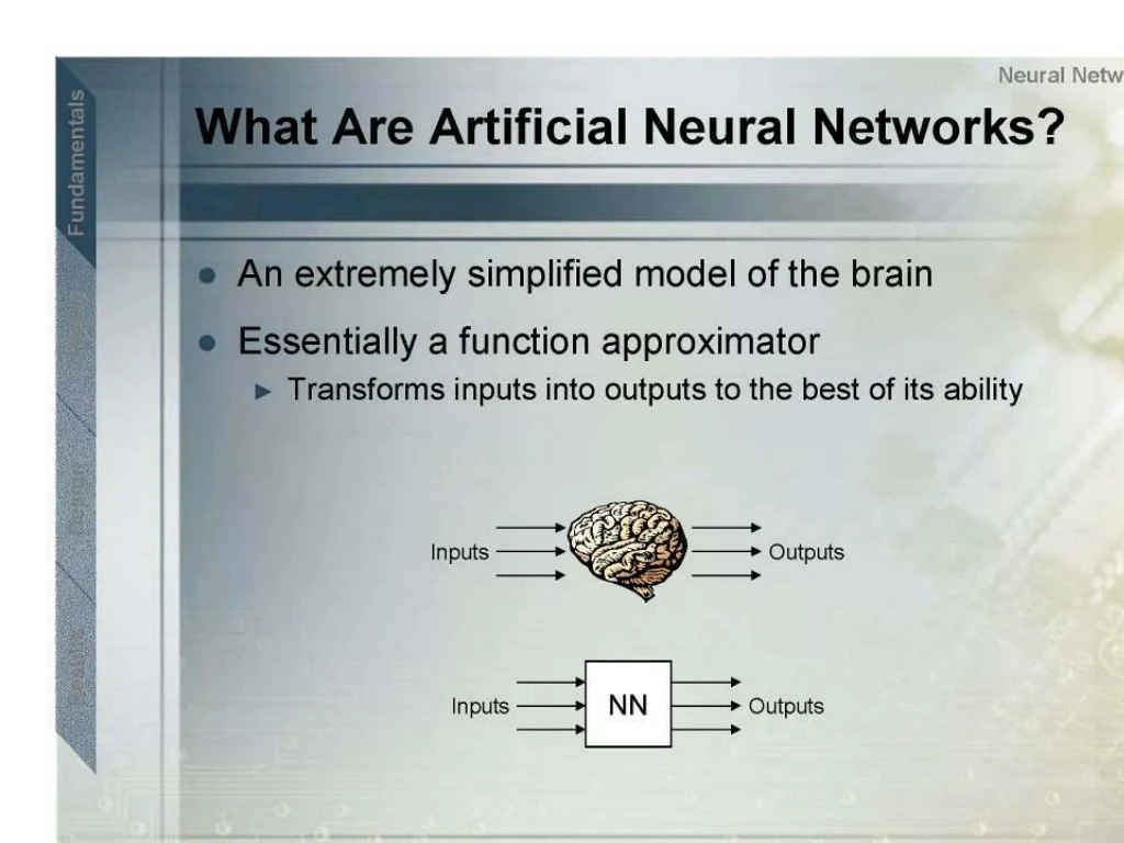
What’s the idea? • assembly of interconnected processing elements • links modified through training magic! magic! problem solution input weighted link output neuron
von Neumann vs. Neural Net CPU data and instructions data data data memory
A few terms • architecture • the variables & their topological relationships • activity rule • specifies how a neuron will respond to its inputs (short time scale) • learning rule • specifies how a neuron will modify itself over longer time scale • supervised neural network • networks that are given ‘training sets’ – a set of inputs and correct answers to learn from • unsupervised neural network • networks that are given only a set of examples to memorize
w0 x1 x2 … xi w1 w2 y wi Single neuron • architecture: • inputs xi • output y • weights wi
w0 x1 x2 … xi w1 w2 y wi Single neuron • activity rule in 2 steps: • neuron activation: • activation function (pick one!): Deterministic options Stochastic options
w0 x1 x2 … xi w1 w2 y wi Single neuron • learning rule: • compute error signal, or difference between target and output: • adjust the weights accordingly: • or batch learning: stuff all the input / target sets through the neuron and then modify the weight
Binary Hopfield Network • architecture: I neurons with symmetric, bidirectional connections and weights wij • activity rule: • may be synchronous, asynchronous, or even continuous • learning rule: each memory should be a stable state of the network’s activity rule. e.g. Hebb rule:
Hopfield Network Memory & Capacity • more memories: • 5 gives stable but shallow states • 6 results in disaster: • maximum number of patterns with ‘total’ stability criterion • Avalanche occurs at
Perceptron Training • Assume supervised training examples giving the desired output for a unit given a set of known input activations. • Learn synaptic weights so that unit produces the correct output for each example. • Perceptron uses iterative update algorithm to learn a correct set of weights.
Perceptron Learning Rule • Update weights by: where η is the “learning rate” tj is the teacher specified output for unit j. • Equivalent to rules: • If output is correct do nothing. • If output is high, lower weights on active inputs • If output is low, increase weights on active inputs • Also adjust threshold to compensate:
Perceptron Learning Algorithm • Iteratively update weights until convergence. • Each execution of the outer loop is typically called an epoch. Initialize weights to random values Until outputs of all training examples are correct For each training pair, E, do: Compute current output oj for E given its inputs Compare current output to target value, tj , for E Update synaptic weights and threshold using learning rule
Perceptron as a Linear Separator • Since perceptron uses linear threshold function, it is searching for a linear separator that discriminates the classes. o3 ?? Or hyperplane in n-dimensional space o2
Hill-Climbing in Multi-Layer Nets • Since “greed is good” perhaps hill-climbing can be used to learn multi-layer networks in practice although its theoretical limits are clear. • However, to do gradient descent, we need the output of a unit to be a differentiable function of its input and weights. • Standard linear threshold function is not differentiable at the threshold. oi 1 0 Tj netj
Differentiable Output Function • Need non-linear output function to move beyond linear functions. • A multi-layer linear network is still linear. • Standard solution is to use the non-linear, differentiable sigmoidal “logistic” function: 1 0 Tj netj Can also use tanh or Gaussian output function
Backpropagation Learning Rule • Each weight changed by: where η is a constant called the learning rate tj is the correct teacher output for unit j δj is the error measure for unit j
Update weights into j Error Backpropagation • First calculate error of output units and use this to change the top layer of weights. Current output: oj=0.2 Correct output: tj=1.0 Error δj = oj(1–oj)(tj–oj) 0.2(1–0.2)(1–0.2)=0.128 output hidden input
Error Backpropagation • Next calculate error for hidden units based on errors on the output units it feeds into. output hidden input
Update weights into j Error Backpropagation • Finally update bottom layer of weights based on errors calculated for hidden units. output hidden input
Backpropagation Training Algorithm Create the 3-layer network with H hidden units with full connectivity between layers. Set weights to small random real values. Until all training examples produce the correct value (within ε), or mean squared error ceases to decrease, or other termination criteria: Begin epoch For each training example, d, do: Calculate network output for d’s input values Compute error between current output and correct output for d Update weights by backpropagating error and using learning rule End epoch
Comments on Training Algorithm • Not guaranteed to converge to zero training error, may converge to local optima or oscillate indefinitely. • However, in practice, does converge to low error for many large networks on real data. • Many epochs (thousands) may be required, hours or days of training for large networks. • To avoid local-minima problems, run several trials starting with different random weights (random restarts). • Take results of trial with lowest training set error. • Build a committee of results from multiple trials (possibly weighting votes by training set accuracy).