Download
1 / 84
840 likes | 863 Views
This course provides insight into viscous fluid flow phenomena, deriving governing equations and applying boundary layer theory for practical cases.

E N D
Course Number: 804538 Advance Fluid Mechanics Faculty Name Prof. A. A. Saati
804538 Advanced Fluid Mechanics • Course Number: 804538 • Course Title: Advanced Fluid Mechanics • Credit ( Lec, Lab, Cr ): (3, 0, 3) • Prerequisite: 804305 or A. C. • Course Objective: This course gives the students insight into the phenomena of viscous fluid flow, to enable them derive the governing equations for practical cases and to show how the boundary layer theory can make flows involving fluids of small viscosity amenable to successful theoretical analysis
804538 Advanced Fluid Mechanics • Course Outline: • Conservation equations for viscous fluids – • boundary layer concept – • Navier-Stokes equation and some exact solutions – • Laminar boundary layer equations and methods of solution • Von Karman momentum integral equation – • Theory of stability of laminar flows – • Introduction to turbulent flow.
Lecture # 1 Chapter: 1 Fundamentals Ref. ADVANCED FLUID MECHANICS By W. P. Graebel
1.1 Introduction • The fundamentals laws of fluid mechanics: • conservation of mass • Newton's laws, and • the laws of thermodynamics
1.1 Introduction • The quantitiesof mass, momentum and energy for a given volume of fluid mechanics will change due to: • internal causes • net change in that quantity entering and leaving • action on the surface
In some cases a global description (by applying the basic laws) is satisfactory for carrying out further analysis, but • A local statement of the laws in the form of differential equations is preferred to obtain more detailed information on the behavior of the quantity.
Divergence theorem is a way to convert certain types of surface integrals to volume integrals • Where: • The theoremassumesthat the scalar and vector quantities are finite and continuous within V and on S.
In studying fluid mechanic three laws can be expressed in the following descriptive form:
The general term used to classify the fluid mechanic quantities is tensor. • The orderof a tensor refers to the number of directions associated with the term: • Example: • pressure and temperature, have magnitude but zero directional property • Velocity, have magnitude but one direction associated with them • Stress, have magnitude but two directions associated with them
To qualify as a tensor, quantity must have more than the magnitude and directionality. • When the components of the tensor are comperedin two coordinate systems that have origins at the same point, the components must relate one another in a specific manner. • Example: • Tensor of order zero, the transformation law is simply that the magnitude are the same in both coordinate systems • Tensor of order one, must transform according to the parallelogram law (the component in one coordinate system are the sum of products of direction cosines of the angles between the two sets of axes and the components in the second system).
Cartesian coordinates • When dealing with flows that involve flat surfaces. • Boundary conditions are most easily satisfied, manipulation are easiest,…… • The components of a vector are represented by:
1.2 Velocity, Acceleration, and the Material Derivative • A fluid is defined as material that will undergo constant motion when shearing forces are applied, the motion continuing as long as the sheering forces are maintained.
1.2 Velocity, Acceleration, and the Material Derivative • Velocity of the particle is given by:
1.2 Velocity, Acceleration, and the Material Derivative • Acceleration of the particle is given by: • Notes: that the are fixed for the partial derivatives
1.2 Velocity, Acceleration, and the Material Derivative • Eularian or spatial description • The velocity is written as , Where x refers to the position of a fixed point in space, as the basic descriptor rather than displacement. • The acceleration component in the x direction is defined as:
1.2 Velocity, Acceleration, and the Material Derivative • Eularian or spatial description • Similar results for acceleration component in the y and z direction is defined as: • And the vector form is defined as:
1.2 Velocity, Acceleration, and the Material Derivative • Eularian or spatial description • The first term is referred to the temporal acceleration, and the secondas convective or advective, acceleration. • The convectiveterm can also be written as
1.2 Velocity, Acceleration, and the Material Derivative • Eularian or spatial description • Material or substantial derivative • represents differentiation as fluid partial is • monitored • Note that is not correct vector operator.
1.3 The Local Continuity Equation • A Control volume is a device used in analyzing fluid flows to account for mass, momentum, and energy balance • A control surface is the bounding surface of the control volume. • The mass of the fluid inside our control volume is • The rate of change of mass inside of our control volume is • (for fixed VC in space) • The rate of change of mass inside of our control volume through its surface dSis
1.3 The Local Continuity Equation • The net rate of change of mass inside and entering the control volume and setting the sum to zero is given by • Transform the surface integral to a volume integral • Making this replacement in the above equation
1.3 The Local Continuity Equation • Since the choice of the control volume was arbitrary and since the integral must vanish no matter what choice of control volume was made, the only way this integral can vanish is for the integrand to vanish
1.3 The Local Continuity Equation • An incompressible is defined as one where the mass density of the fluid particle does not change as the particle followed
1.4 Path Line, Streamline and Stream Function • A path line is a line along which a fluid particle actually travels. • Since the particle incrementally moves in the direction of the velocity vector, the equation of a path line is given by • Note : the integration being performed with held fixed • A streamline is defined as line drawn in the flow at a given instant of time such that the fluid velocity vector at any point in the streamline is tangent to the line at that point.
1.4 Path Line, Streamline and Stream Function • A streamline is defined as line drawn in the flow at a given instant of time such that the fluid velocity vector at any point in the streamline is tangent to the line at that point. • The streamline are given by equation • A stream surface is a collection of adjacent streamlines, providing a surface through which there is no flow • A stream tube is a tube made up of adjoining streamlines
1.4 Path Line, Streamline and Stream Function • For steady flows the path lines and streamlines overlap • For unsteady flows the path lines and streamlines may differ • Stream functions are used mainly in connection with incompressible flows (where the density of individual particle does not change) and the equation reduce to
1.4.1 Lagrange’s Stream Function for Tow-Dimensional Flows • For 2-D flows equation reduces to • Integrating that one of the velocity components can be expressed in tem of the other. • Lagrange’s stream function is a scalar function , and expressing the two velocity in terms of .
1.4.1 Lagrange’s Stream Function for Tow-Dimensional Flows • In 2-D the tangency requirement equation • Using the expression of velocity in term of stream function • This equation states that along a streamline vanishes, and is constant. • The suitable expressions for the velocity component in cylindrical polar coordinates are
1.4.2 Stream Function for Three-Dimensional Flows • For 3-D equation states that there is one relationship between the three velocity components • So it is expected that the velocity can be expressed in terms of two scalar function • The clarification of stream function as introduced in two dimensions is • Where and are each constant on stream surfaces.
1.4.2 Stream Function for Three-Dimensional Flows • A particular three dimensional case in which a stream function is useful is that of axisymmetric flow. • Taking the z-axis as the axis of symmetry: • Spherical polar coordinates • Cylindrical polar coordinates
1.4.2 Stream Function for Three-Dimensional Flows • Since any plane given by equal to constant is therefore a stream function given by • Spherical polar coordinates • Cylindrical polar coordinates
1.5 Newton’s Momentum Equation • Themomentumin the interior of the control volume is • Therate at which momentum enters the control volume through its surface is • Thenet rate of change of momentum is then
1.5 Newton’s Momentum Equation • The forces applied to the surface of the control volume are due to • Pressure force • Viscous force • Gravity force • The net force is then • The net change in momentum gives • Using the divergence theorem, this reduce to
1.6 Stress • Stress is defined as force applied to an area • Consider the three special stress vectors corresponding to forces acting on areas unit normal pointing in the x, y, z, directions (n=i, n=j, n=k)
1.6 Stress • In the limit, as the areas are taken smaller and smaller, the forces acting are • Where acting on -x, -y, -z, directions • And • The summing result is • In limiting the areas goes to zero
1.6 Stress • Combine the above equations (*) & (**) • Integrate the above equation and change the surface integral to volume integral
1.6 Stress • Integrate the above equation and change the surface integral to volume integral
1.6 Stress • Integrate the above equation The net change in momentum equation gives • As was the case for continuity equation, the above equation must be valid no matter what volume we choose • Therefore, it must be that
Stress vector Stress tensor
1.6 Stress • The continuity equation and The momentum equation in (11) can be written in a matrix form as • This form referred to as conservation form and frequently used in computational fluid dynamic
1.6 Stress • Momentscan be balanced in the same manner as forces • Using a finite control mass and taking R as a position vector drawn from the point about which moments are being taken • From equations (2) &(4) {ppt 36}; • The time rate of change of moment of momentum is given by
1.6 Stress • And using the product rule • Also using the product rule to develop • The surface integral
1.6 Stress • Thus, using equations (14, 15, 16, 17) in equation (13)
1.7 Rates of Deformation • Rate of deformation is the quantity that describes the fluids’ behavior under stress. • Select points A,B,C, to make up a right angle at an initial time t • At later time , these points will have moved to A’,B’, and C’ • Point A will have x and y velocity components
1.7 Rates of Deformation • Point A will have x and y velocity components • And will move a distance • Similarly for point B&C to B’&C’