Download
1 / 30
300 likes | 402 Views
GLOBAL MODELS OF ATMOSPHERIC COMPOSITION Daniel J. Jacob Harvard University. HOW TO MODEL ATMOSPHERIC COMPOSITION? Solve continuity equation for chemical mixing ratios C i ( x , t). U = wind vector P i = local source of chemical i L i = local sink. Eulerian form:. Lightning.

E N D
GLOBAL MODELS OF ATMOSPHERIC COMPOSITIONDaniel J. JacobHarvard University
HOW TO MODEL ATMOSPHERIC COMPOSITION?Solve continuity equation for chemical mixing ratios Ci(x, t) U = wind vector Pi= local source of chemical i Li = local sink Eulerian form: Lightning Lagrangian form: Transport Chemistry Aerosol microphysics Human activity Volcanoes Fires Land biosphere Ocean
EULERIAN MODELS PARTITION ATMOSPHERIC DOMAIN INTO GRIDBOXES This discretizes the continuity equation in space Solve continuity equation for individual gridboxes • Detailed chemical/aerosol models can presently afford -106 gridboxes • In global models, this implies a horizontal resolution of ~ 1o (~100 km) in horizontal and ~ 1 km in vertical • Chemical Transport Models (CTMs) use external meteorological data as input • General Circulation Models (GCMs) compute their own meteorological fields
Reduces dimensionality of problem OPERATOR SPLITTING IN EULERIAN MODELS • Split the continuity equation into contributions from transport and local terms: … and integrate each process separately over discrete time steps: • These operators can be split further: • split transport into 1-D advective and turbulent transport for x, y, z • (usually necessary) • split local into chemistry, emissions, deposition (usually not necessary)
SPLITTING THE TRANSPORT OPERATOR • Wind velocity U has turbulent fluctuations over time step Dt: Time-averaged component (resolved) Fluctuating component (stochastic) • Split transport into advection (mean wind) and turbulent components: advection turbulence (1st-order closure) • Further split transport in x, y, and z to reduce dimensionality. In x direction: turbulent operator advection operator
SOLVING THE EULERIAN ADVECTION EQUATION • Equation is conservative: need to avoid diffusion or dispersion of features. Also need mass conservation, stability, positivity… • All schemes involve finite difference approximation of derivatives : order of approximation → accuracy of solution • Classic schemes: leapfrog, Lax-Wendroff, Crank-Nicholson, upwind, moments… • Stability requires Courant number uDt/Dx < 1 • … limits size of time step • Addressing other requirements (e.g., positivity) introduces non-linearity in advection scheme
generally dominates over mean vertical advection • K-diffusion OK for dry convection in boundary layer (small eddies) • Deeper (wet) convection requires non-local convective parameterization VERTICAL TURBULENT TRANSPORT (BUOYANCY) Convective cloud (0.1-100 km) Wet convection is subgrid scale in global models and must be treated as a vertical mass exchange separate from transport by grid-scale winds. Need info on convective mass fluxes from the model meteorological driver. detrainment Model vertical levels downdraft updraft entrainment Model grid scale
LOCAL (CHEMISTRY) OPERATOR:solves ODE system for n interacting species For each species System is typically “stiff” (lifetimes range over many orders of magnitude) → implicit solution method is necessary. • Simplest method: backward Euler. Transform into system of n algebraic equations with n unknowns Solve e.g., by Newton’s method. Backward Euler is stable, mass-conserving, flexible (can use other constraints such as steady-state, chemical family closure, etc… in lieu of DC/Dt ). But it is expensive. Most 3-D models use higher-order implicit schemes such as the Gear method.
SPECIFIC ISSUES FOR AEROSOL CONCENTRATIONS • A given aerosol particle is characterized by its size, shape, phases, and chemical composition – large number of variables! • Measures of aerosol concentrations must be given in some integral form, by summing over all particles present in a given air volume that have a certain property • If evolution of the size distribution is not resolved, continuity equation for aerosol species can be applied in same way as for gases • Simulating the evolution of the aerosol size distribution requires inclusion of nucleation/growth/coagulation terms in Piand Li, and size characterization either through size bins or moments. Typical aerosol size distributions by volume coagulation condensation nucleation
LAGRANGIAN APPROACH: TRACK TRANSPORT OF POINTS IN MODEL DOMAIN (NO GRID) • Transport large number of points with trajectories from input meteorological data base (U) + random turbulent component (U’) over time steps Dt • Points have mass but no volume • Determine local concentrations as the number of points within a given volume • Nonlinear chemistry requires Eulerian mapping at every time step (semi-Lagrangian) position to+Dt U’Dt • PROS over Eulerian models: • no Courant number restrictions • no numerical diffusion/dispersion • easily track air parcel histories • invertible with respect to time • CONS: • need very large # points for statistics • inhomogeneous representation of domain • convection is poorly represented • nonlinear chemistry is problematic UDt position to
LAGRANGIAN RECEPTOR-ORIENTED MODELING Run Lagrangian model backward from receptor location, with points released at receptor location only • Efficient cost-effective quantification of source influence distribution on receptor (“footprint”) • Enables inversion of source influences by the adjoint method (backward model is the adjoint of the Lagrangian forward model)
EMBEDDING LAGRANGIAN PLUMES IN EULERIAN MODELS Release puffs from point sources and transport them along trajectories, allowing them to gradually dilute by turbulent mixing (“Gaussian plume”) until they reach the Eulerian grid size at which point they mix into the gridbox S. California fire plumes, Oct. 25 2004 • Advantages: resolve subgrid ‘hot spots’ and associated nonlinear processes (chemistry, aerosol growth) within plume • Difference with Lagrangian approach is that (1) puff has volume as well as mass, (2) turbulence is deterministic (Gaussian spread) rather than stochastic
GEOS-Chem GLOBAL 3-D CHEMICAL TRANSPORT MODEL • Solves 3-D continuity equations on global Eulerian grid using NASA Goddard Earth Observing System (GEOS) assimilated meteorological data (1985-present) or GISS GCM output (paleo and future climate) • Horizontal resolution 1ox1o to 4ox5o, 48-72 vertical layers • Used by ~30 groups around the world for wide range of atmospheric composition problems: aerosols, oxidants, carbon, mercury, isotopes… Illustrate here with Harvard work on tropospheric ozone
OZONE: “GOOD UP HIGH, BAD NEARBY” • Nitrogen oxide radicals; NOx = NO + NO2 • Sources: combustion, soils, lightning • Volatile organic compounds (VOCs) • Methane • Sources: wetlands, livestock, natural gas… • Non-methane VOCs (NMVOCs) • Sources: vegetation, combustion • Carbon monoxide (CO) • Sources: combustion, VOC oxidation Tropospheric ozone precursors
RADICAL CYCLE CONTROLLING TROPOSPHERIC OH AND OZONE CONCENTRATIONS GEOS-Chem simulation for tropospheric ozone includes 120 coupled species to describe HOx-NOx-VOC-aerosol chemistry O2 hn O3 STRATOSPHERE 8-18 km 400 TROPOSPHERE global sources/sinks in Tg y-1 4300 hn NO2 NO O3 hn, H2O OH HO2 H2O2 4000 Deposition 700 CO, VOCs SURFACE
Climatology of observed ozone at 400 hPa in July from ozonesondes and MOZAIC aircraft (circles) and corresponding GEOS-Chem model results for 1997 (contours). GLOBAL DISTRIBUTION OF TROPOSPHERIC OZONE GEOS-Chem tropospheric ozone columns for July 1997. Li et al., JGR [2001]
COMPARISON TO TES SATELLITE OBSERVATIONS IN MIDDLE TROPOSPHERE (July 2005) averaging kernels Zhang et al. [2006]
TES ozone and CO observations in July 2005 at 618 hPa North America Asia TES observations of ozone-CO correlations test GEOS-Chem simulation of ozone continental outflow Zhang et al., 2006
GEOS-Chem GLOBAL BUDGET OF TROPOSPHERIC OZONE Present-day Preindustrial O2 hn O3 STRATOSPHERE 8-18 km TROPOSPHERE hn NO2 NO O3 hn, H2O OH HO2 H2O2 Deposition CO, VOC
IPCC RADIATIVE FORCING ESTIMATE FOR TROPOSPHERIC OZONE (0.35 W m-2) RELIES ON GLOBAL MODELS …but these underestimate the observed rise in ozone over the 20th century Preindustrial ozone models } Observations at mountain sites in Europe [Marenco et al., 1994]
RADIATIVE FORCING BY TROPOSPHERIC OZONE COULD THUS BE MUCH LARGER THAN IPCC VALUE Global simulation of late 19th century ozone observations [Mickley et al., 2001] Standard model: DF = 0.44 W m-2 “Adjusted” model (lightning and soil NOx decreased, biogenic hydrocarbons increased): DF = 0.80 W m-2
IMPLICATION OF RISING BACKGROUND FOR MEETING AIR QUALITY STANDARDS Europe AQS (8-h avg.) Europe AQS (seasonal) U.S. AQS (8-h avg.) U.S. AQS (1-h avg.) 0 20 40 60 80 100 120 ppbv Preindustrial ozone background Present-day ozone background at northern midlatitudes Shutting down N. American anthropogenic emissions in GEOS-Chem reduces frequency of European exceedances of 55 ppbv standard by 20%
The U.S. EPA defines a “policy-relevant background” (PRB) as the ozone concentration that would be present in U.S. surface air in the absence of N. American anthropogenic emissions • This background cannot be directly observed, must be estimated from models • Because chemistry is strongly nonlinear, sensitivity simulations are necessary • Standard simulation; include all sources • (2) Set U.S. or N. American anthropogenic emissions to zero a infer policy-relevant background • (3) Set global anthropogenic emissions to zero a estimate natural background • Difference between (1) and (2) a regional pollution • Difference between (2) and (3) a background enhancement from hemispheric pollution
Summer 1995 afternoon (1-5 p.m.) ozone in surface air over the U.S. Observations GEOS-CHEM standard simulation r = 0.66, bias=5 ppbv Fiore et al. [2002]
High-O3 events: dominated by regional pollution; minor stratospheric influence (~2 ppbv) regional pollution hemispheric pollution * CASTNet observations Model Background Natural O3 level Stratospheric } Regional pollution D = Examine a clean site: Voyageurs National Park, Minnesota(May-June 2001) } D = Hemispheric pollution + X Background: 15-36 ppbv Natural level: 9-23 ppbv Stratosphere: < 7 ppbv Fiore et al. [2003]
Compiling daily afternoon (1-5 p.m. mean) surface ozone from all CASTNet rural sites for March-October 2001: Policy-relevant background ozone is typically 20-35 ppbv Natural 18±5 ppbv GEOS-Chem PRB 26±7 ppbv GEOS-Chem PRB 29±9 ppbv MOZART-2 Probability ppbv-1 CASTNet sites GEOS-Chem Model at CASTNet Fiore et al., JGR 2003
2000 2050 climate - 2000 EFFECT OF 2000-2050 CLIMATE CHANGE ON U.S. OZONE POLLUTION Run GEOS-Chem driven by GISS GCM for present vs. 2050 climate • Climate change decreases the background ozone because higher water vapor increases ozone loss; • but it aggravates ozone pollution episodes due to less ventilation (fewer • mid-latitudes cyclones), faster chemistry, higher biogenic VOC emissions Wu et al. [2007]
CONSTRAINING NOx AND REACTIVE VOC EMISSIONS WITH NO2 AND FORMALDEHYDE (HCHO) MEASUREMENTS FROM SPACE GOME: 320x40 km2 SCIAMACHY: 60x30 km2 OMI: 24x13 km2 Tropospheric NO2 column ~ ENOx Tropospheric HCHO column ~ EVOC ~ 2 km hn (420 nm) BOUNDARY LAYER hn (340 nm) NO2 NO HCHO CO OH hours O3, RO2 hours VOC 1 day HNO3 Emission Deposition Emission VOLATILE ORGANIC COMPOUNDS (VOC) NITROGEN OXIDES (NOx)
TOP-DOWN CONSTRAINTS ON NOx EMISSION INVENTORIESFROM OMI NO2 DATA INTERPRETED WITH GEOS-Chem Boersma et al. [2007] Tropospheric NO2 (March 2006) OMI – GEOS-Chem difference OMI observations GEOS-Chem with EPA 1999 emissions • Fitting OMI NO2 with GEOS-Chem requires • 25% decrease in power plant emissions • 30% increase in vehicle emissions • relative to EPA 1999 official inventory
FORMALDEHYDE COLUMNS FROM OMI (Jun-Aug 2006): high values are due to biogenic isoprene (main reactive VOC) GEOS-Chem model w/best prior (MEGAN) biogenic VOC emissions OMI MEGAN emission hot spots not substantiated by the OMI data Millet et al. [2007]