Download
1 / 44
440 likes | 466 Views
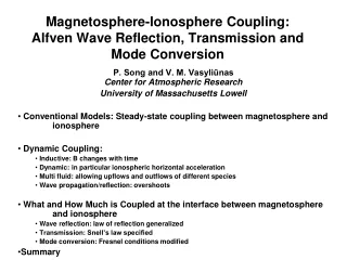
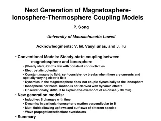
Next Generation of Magnetosphere-Ionosphere-Thermosphere Coupling Models. P. Song University of Massachusetts Lowell Acknowledgments: V. M. Vasyliūnas, and J. Tu Conventional Models: Steady-state coupling between magnetosphere and ionosphere

E N D
Next Generation of Magnetosphere-Ionosphere-Thermosphere Coupling Models P. Song University of Massachusetts Lowell Acknowledgments: V. M. Vasyliūnas, and J. Tu Conventional Models: Steady-state coupling between magnetosphere and ionosphere (Steady state) Ohm’s law with constant conductivities Electrostatic potential Constant magnetic field: self-consistency breaks when there are currents and spatially varying electric field Dynamics in the magnetosphere does not couple dynamically to the ionosphere Ionospheric horizontal motion is not derived with dynamic effects Observationally, difficult to explain the overshoot of an onset (< 30 min) New generation models: Inductive: B changes with time Dynamic: in particular ionospheric motion perpendicular to B Multi fluid: allowing upflows and outflows of different species Wave propagation/reflection: overshoots Summary
M-I Coupling • Explain the observed ionospheric responses to solar wind condition/changes, substorms and auroras etc. and feedback to the magnetosphere (not to simply couple codes) • Conventional: Ohm’s law in the neutral frame=> the key to coupling • Derived from steady state equations (no ionospheric acceleration) • Conductivities are time constant • J and E are one-to-one related: no dynamics • Magnetospheric Approach • Height-integrated ionosphere • Neutral wind velocity is not a function of height and time • Ionospheric Approach • Structured ionosphere • Magnetosphere is a prescribed boundary • Not self-consistent: steady state equations to describe time dependent processes (In steady state, imposed E-field penetrates into all heights) • Do not solve Maxwell equations
Field-aligned Current Coupling Models Full dynamics Electrostatic Steady state (density and neutrals time varying) • coupled via field-aligned current, closed with Pedersen current • Ohm’s law gives the electric field and Hall current • electric drift gives the ion motion
M-I Coupling (Conventional) • Ohm’s law in the neutral frame: the key to coupling • Magnetospheric Approach • Height-integrated ionosphere • Current conservation • Neutral wind velocity is not a function of height and time • No self-consistent field-aligned flow • No ionospheric acceleration • Ionospheric Approach • Structured ionosphere • Magnetosphere is a prescribed boundary • Not self-consistent: steady state equations to describe time dependent processes (In steady state, imposed E-field penetrates into all heights) • Do not solve Maxwell equations
M-I coupling model: Driven by imposed E-field in the polar cap
M-I Coupling (Conventional) • Ohm’s law in the neutral frame: the key to coupling • Magnetospheric Approach • Height-integrated ionosphere • Neutral wind velocity is not a function of height and time • Ionospheric Approach • Structured ionosphere • Magnetosphere is a prescribed boundary • When upper boundary varies with time, the ionosphere varies with time: (misinterpreted as dynamic coupling) • Not self-consistent: steady state equations to describe time dependent processes (In steady state, imposed E-field penetrates into all heights) • Do not solve Maxwell’s equations • No wave reflection • No fast and slow modes in ionosphere (force imbalance cannot propagate horizontally) • No ionospheric acceleration
Theoretical Basis for Conventional Coupling Models • B0 >>δB and B0 is treated as time independent in the approach, and δB is produced to compare with observations • not a bad approximation • questionable for short time scales: dynamics • questionable for short time scales • Time scale to reach quasi-steady state δt~δLδB/δE • given δL, from the magnetopause to ionosphere, 20 Re • δB, in the ionosphere, 1000 nT • δE, in the ionosphere, for V~1 km/s, 6x10⁻² V/m • δt ~ 2000 sec, 30 min, substorm time scale! • Conventional theory is not applicable to substorms, auroral brightening!
Ionospheric Dynamic Processes Epoch analysis showing on average an overshoot in ionospheric velocity for 30 min. An overshoot lasting 40 min was seen on ground but not in geosynchronous orbits; indicating the overshoot is related to the ionospheric processes Huang et al, 2009
Ion-neutral Interaction • Magnetic field is frozen-in with electrons • Plasma (red dots) is driven with the magnetic field (solid line) perturbation from above • Neutrals do not directly feel the perturbation while plasma moves • Ion-neutral collisions accelerate neutrals (open circles), strong friction/heating • Longer than the neutral-ion collision time, the plasma and neutrals move nearly together with a small slippage. Weak friction/heating • On very long time scales, the plasma and neutrals move together: no collision/no heating
Ionosphere Reaction to Magnetospheric Motion • Slow down wave propagation (neutral inertia loading) • Partial reflection • Drive ionosphere convection • Large distance at the magnetopause corresponds to small distance in the ionosphere • In the ionosphere, horizontal perturbations propagate in fast mode speed • Ionospheric convection modifies magnetospheric convection (true 2-way coupling)
Global Consequence of A Poleward Motion • Antisunward motion of open field line in the open-closed boundary creates • a high pressure region in the open field region (compressional wave), and • a low pressure region in the closed field region (rarefaction wave) • Continuity requirement produces convection cells through fast mode waves in the ionosphere and motion in closed field regions. • Poleward motion of the feet of the flux tube propagates to equator and produces upward motion in the equator. • Ionospheric convection will drive/modify magnetospheric convection
Expected Heating Distribution • For uniform conductivity, velocity pattern coincides with the magnetic perturbation. • FAC forms at the center of the convection cells • Poynting flux is proportional to V2, weakest at the center of convection cells • Neglecting the heating from precipitation particles, • Conventional model (EJ paradigm) predicts heating, J2/p, is highest at the FAC • New model (BV paradigm) predicts heating, iniV2, is highest at compression region of dayside and nightside cusps and strong along the noon-midnight meridian sun
Consequence of Heating • Energy equation • Neglecting radiative loss, R, and heat conduction • Enhanced temperature and upward motion are expected
Basic Equations • Continuity equations • Momentum equations • Temperature equations • Faraday’s Law and Ampere's Law s = e, i or n, and es = -e, e or 0 Field-aligned flow allowed
Simplifying Assumptions (dt > 1sec) • Charge quasi-neutrality • Replace electron continuity with • Neglecting the electron inertial term in the electron momentum equation • Electric field, E, can be eliminated in other equations; • electron velocity will be calculated from current definitions.
Numeric Consideration Large collision frequencies make equations strongly stiff is very large at low altitude, e.g., at 80 km s-1 Extremely small time step (< 10-6 s) is required for explicit algorithms to be numerically stable. Implicit algorithms are necessary
1-D Stratified Ionosphere/thermosphere • Equation set is solved in 1-D (vertical), assume B<<B0. • Neutral wind velocity is a function of height and time • The system is driven by a change in the motion at the top boundary • No local field-aligned current; horizontal currents are derived • No imposed E-field; E-field is derived. • test 1: solve momentum equations and Maxwell’s equations using explicit method • test 2: use implicit method (increasing time step by 105 times) • test 3: include continuity and energy equations with field-aligned flow 2000 km 500 km
Dynamics in 2-Alfvén Travel Time x: antisunward; y: dawnward, z: upward, B0: downward On-set time: 1 sec Several runs were made: the processes are characterized in Alfvén time Building up of the Pedersen current Song et al., 2009
30 Alfvén Travel Time • The quasi-steady state is reached in ~ 20 Alfvén time. • During the transition, antisunward flow in the F-layer can be large • During the transition, E-layer and F-layer have opposite dawn-dusk flows • There is a current enhancement for ~10 A-time, more in “Pedersen” current Song et al., 2009
Neutral wind velocity • The neutral wind driven by M-I coupling is strongest in F-layer • Antisunward wind continues to increase Song et al., 2009
After 1 hour, a flow reversal at top boundary • Antisunward flow reverses and enhances before settled • Dawn-dusk velocity enhances before reversing (flow rotates) • The reversal transition takes slightly longer than initial transition • Larger field fluctuations Song et al., 2009
After 1 hour, a flow reversal at top boundary “Pedersen” current more than doubled just after the reversal Song et al., 2009
Electric field variationsNot Constant! Electric field in the neutral wind frame E’ = E + unxB Not Constant! Song et al., 2009
Heating rate q as function of Alfvén travel time and height. The heating rate at each height becomes a constant after about 30 Alfvén travel times. The Alfvén time is the time normalized by tA, which is defined as If the driver is at the magnetopause, the Alfvén time is about 1 min. Height variations of frictional heating rate and true Joule heating rate at a selected time. The Joule heating rate is negligibly small. The heating is essentially frictional in nature. Tu et al., 2011
Heating rate divided by total mass density (neutral mass density plus plasma mass density) as function of Alfvén travel time and height. The heating rate per unit mass is peaked in the F layer of the ionosphere, around about 300 km in this case. Time variation of height integrated heating rate. After about 30 Alfvén travel times, the heating rate reaches a constant. This steady-state heating rate is equivalent to the steady-state heating rate calculated using conventional Joule heating rate J∙(E+unxB) defined in the frame moving with the neutral wind. In the transition period, the heating rate can be two times larger than the steady-state heating rate. Tu et al., 2011
Summary • A new scheme of solar wind-magnetosphere-ionosphere-thermosphere coupling is proposed • Including continuity, momentum equation, and energy equation for each species of multi fluids • Including Maxwell’s equations • Including photochemistry • No imposed E-field is necessary, and no imposed field-aligned current is necessary • 1-D studies: steady state, wave dispersion relation and attenuation, time dependence, ionospheric heating, coronal heating • An implicit numerical scheme has been developed to make the time step large (5 orders) enough for global simulations • In 1-D simulations, there are 4 major differences between the dynamic (and inductive) coupling and the steady-state coupling • Transient time for M-I equilibrium: not Alfvén travel time, but 10-20 tA ~ 20-30 min. • Reflection effect: enhanced Poynting flux and heating rate during the dynamic transient period can be a factor of 1.5 greater than that given in of steady-state coupling • Plasma inertia effect: velocity, magnetic field, and electric field perturbations depend on density profile during the transition period • Field-aligned upflow allowed • In 2-D and 3-D: ionosphere can be an active player in determining magnetospheric convection. It can be the driver in some regions. • Using Ohm’s law in the neutral wind frame in conventional M-I coupling will miss • the dynamics during the transition < 30 min • neutral wind acceleration > 1 hr.
Comparison of Steady-state Coupling with Dynamic Coupling • Coupling speed Vphase • Steady-state Coupling • Original model (Vasyliunas, 1970, Wolf, 1970): not specific, presumed to be VA • Implemented in simulations: (instantaneously) • Dynamic Coupling: Vphase ~ α1/2 VA( is neutral inertia loading factor) • Coupling time δt • Steady-state Coupling • Original model: not specified, • Implemented in simulations: ~0 • Dynamic Coupling: 1~2 min (Alfvén transient) 30 min (M-I equilibrium) 1~3 hours (neutral acceleration)
Comparison of Steady-state Coupling with Dynamic Coupling, cont. • Reflection • Steady-state Coupling • Original model: Multiple reflections assumed, V,B = final result, (depends on ionospheric conductivity) • Implemented in simulations: No reflection, E=Einc, V and δB are derived • Dynamic Coupling: Total=I+R for both δB and V • Reflection coefficient γ: depends on gradient (height) and frequency (time lapse); • Reflection may be produced continuously over height • Incident perturbation may consist of a spectrum: dispersion effect • A phase delay φ due to propagation to and from the reflection point
Comparison of Steady-state Coupling with Dynamic Coupling, cont. • Velocity perturbation V • Steady-state Coupling • Original model: Include final result of multiple reflections • Implemented in simulations: • Dynamic Coupling: For single A-wave, parallel propagation, weakly damped (there are reflected waves)
Comparison of Steady-state Coupling with Dynamic Coupling, cont. • Magnetic perturbation δB • Steady-state Coupling: not included as part of model evolution, calculated from J • Dynamic Coupling: For single A-wave parallel propagation weakly damped (there are reflected waves) Local along B, from B0, V0, δB0, ρi0, • Electric field perturbation E • Steady-state Coupling: • Dynamic Coupling: For single A-wave parallel propagation weakly damped (there are reflected waves) • Dynamic with reflection:
Comparison of Steady-state Coupling and Dynamic Coupling, cont. • Current J • Steady-state Coupling: • Dynamic Coupling: (derived from δB, current continuity satisfied) • Poynting vector S • Steady-state Coupling: Not considered explicitly, DC part included implicitly in dissipation • Dynamic Coupling: For single A-wave parallel propagation weakly damped; • Dynamic with reflection;
Comparison of Steady-state Coupling with Dynamic Coupling, cont. • Heating Rate q • Steady-state Coupling: • Dynamic Coupling: For single A-wave parallel propagation weakly damped; The perturbations include incident and reflected waves
Center for Atmospheric Research of UMass Lowell (http://ulcar.uml.edu) • Staff: 23, (4 faculty, 4 students, 3 posdocs, 4 scientists, 8 regular,) • A new group is joining • Products: • Scientific publications (1 book, and 31 papers in 2011) • Ground-based ionospheric sounders (~ 5 systems/yr, list price ~$0.2 M each) • Data/network services (~ 80 stations worldwide) • Space-borne instrumentation (1 completed operation, 1 under development) • Rockets, balloons instrumentation (new to the center) • Collaborators: AFRL, NASA Goddard, Max Plank Institute, NASA Marshal, Stanford, … • Funding: Air Force, NASA, NSF, International science institutions • Annual revenues: ~3 M • Office space: 12000 sqft • Major projects: • AF Radiation belt remediation $ 2.5 mil • NASA: Space Physics ~ $ 1 mil • NSF: Space Weather $0.6 mil
Space Sciences at the Center for Atmospheric Research • Radio Science • Radio wave transmission in plasma • Radio wave propagation in plasma • Ground penetration radar • Space Weather • Radiation belt remediation • Space weather models: • plasmasphere, • magnetopause, • magnetosheath • Magnetospheric Physics • Magnetosphere-ionosphere coupling • Plasmasphere depletion and refilling • Energetic particles measurements and analyses • ULF wave acceleration of particles • Ionospheric Physics • Ionospheric Reference model • Ionospheric out flow and acceleration • Ionospheric disturbance • Solar Physics and Astrophysics • Chromospheric acceleration • Plasma Physics • High voltage conductor in plasma
Advanced Technology at the Center for Atmospheric Research • RF Technologies • Analog: front-end design (receivers/transmitters), Low/high power amplifiers, filters, Antenna design • Digital: Up/down-converters, Synthesizers, Pulse code modulation, Spectral analysis using FPGA’s and DSP’s, FFTs, filters, FPGA (Altera Stratix and Actel Radiation hardened) • Mixed: AtoD, DtoA • General: Circuit Board design and layout, Power Supply development, Radiation hardened circuit technology • Computer Hardware Technologies • Computer Systems: Embedded Computers (SPARC and Intel), Embedded microcontrollers (PIC) • Enclosures and Backplanes: VME chassis, CompactPCI chassis, Ruggedized and space flight chassis • Computer Software Technologies • Operating Systems: Windows XP, Linux, Embedded Real time OS (RTEMS and VxWorks) • Languages: C++, Java, Assembler (Intel X86, PIC embedded and DSP) • Development Tools • ModelSim Verilog • Altera development suite (Quartus II) • Gnu software development tools
Modern Ionosonde and Transmit Antennameasuring height of the ionosphere and temporal variations Digisonde DPS Transmit antenna
20-m dipole along z 500-m dipoles in spin plane RPI: <10 W radiated power 3 kHz – 3 MHz 300 Hz bandwidth Radio Plasma Imager (RPI) on NASA IMAGE satellite in operation Launched 25 Mar 2000
LORERS transmits radio waves to deplete the radiation particles in radiation belt to protect LEO satellites LORERS Mission AFRL/DARPA Radiation-Belt-Remediation (RBR) high-power transmitter under development at the Center
Jupiter Icy Moons Orbiter (2012) • To explore the three icy moons of Jupiter and investigate their makeup, their history and their potential for sustaining life. • To develop a nuclear reactor and show that it can be processed safely and operated reliably in deep space for long-duration deep space exploration. Planetary Advanced Radio Sounder (PARS) for JIMO mission under development at the Center