Download
1 / 22
220 likes | 250 Views
Magnetosphere-Ionosphere Coupling: Alfven Wave Reflection, Transmission and Mode Conversion. P. Song and V. M. Vasyliūnas Center for Atmospheric Research University of Massachusetts Lowell Conventional Models: Steady-state coupling between magnetosphere and ionosphere Dynamic Coupling:

E N D
Magnetosphere-Ionosphere Coupling: Alfven Wave Reflection, Transmission and Mode Conversion P. Song and V. M. Vasyliūnas Center for Atmospheric Research University of Massachusetts Lowell Conventional Models: Steady-state coupling between magnetosphere and ionosphere Dynamic Coupling: Inductive: B changes with time Dynamic: in particular ionospheric horizontal acceleration Multi fluid: allowing upflows and outflows of different species Wave propagation/reflection: overshoots What and How Much is Coupled at the interface between magnetosphere and ionosphere Wave reflection: law of reflection generalized Transmission: Snell’s law specified Mode conversion: Fresnel conditions modified Summary
M-I Coupling • Explain the observed ionospheric responses to solar wind condition/changes, substorms and auroras etc. and feedback to the magnetosphere (not simply to couple codes) • Conventional: Ohm’s law in the neutral frame=> the key to coupling • Derived from steady state equations (no ionospheric acceleration) • Conductivities are time constant (not including ) • J and E are one-to-one related: no dynamics • Magnetospheric Approach • Height-integrated ionosphere • Neutral wind velocity is not a function of height and time • Ionospheric Approach • Structured ionosphere • Magnetosphere is a prescribed boundary • Not self-consistent: steady state equations to describe time dependent processes (In steady state, imposed E-field penetrates into all heights) • Maxwell’s equations not solved
Field-aligned Current Coupling Models Full dynamics Electrostatic Steady state (density and neutrals time varying) • coupled via field-aligned current, closed with Pedersen current • Ohm’s law gives the electric field and Hall current • electric drift gives the ion motion
M-I Coupling (Conventional) • Ohm’s law in the neutral frame: the key to coupling • Magnetospheric Approach • Height-integrated ionosphere • Current conservation • Neutral wind velocity is not a function of height and time • No self-consistent field-aligned flow • No ionospheric acceleration • Ionospheric Approach • Structured ionosphere • Magnetosphere is a prescribed boundary • Not self-consistent: steady state equations to describe time dependent processes (In steady state, imposed E-field penetrates into all heights) • Maxwell’s equations not solved
M-I coupling model: Driven by imposed E-field in the polar cap
M-I Coupling (Conventional) • Ohm’s law in the neutral frame: the key to coupling • Magnetospheric Approach • Height-integrated ionosphere • Neutral wind velocity is not a function of height and time • Ionospheric Approach • Structured ionosphere • Magnetosphere is a prescribed boundary • When upper boundary varies with time, the ionosphere varies with time: (misinterpreted as dynamic coupling) • Not self-consistent: steady state equations to describe time dependent processes (In steady state, imposed E-field penetrates into all heights) • Maxwell’s equations not solved (J and B are not self consistent) • No wave reflection • No propagation in ionosphere (force imbalance cannot propagate horizontally) • No ionospheric acceleration
Theoretical Basis for Conventional Coupling Models • B0 >>δB and B0 is treated as time independent in the approach, and δB is produced to compare with observations • not a bad approximation • questionable for short time scales: dynamics • questionable for short time scales • Time scale to reach quasi-steady state δt~δLδB/δE • given δL, from the magnetopause to ionosphere, 20 Re • δB, in the ionosphere, 1000 nT • δE, in the ionosphere, for V~1 km/s, 6x10⁻² V/m • δt ~ 2000 sec, 30 min, substorm time scale! • Conventional theory is not applicable to substorms, auroral brightening!
Ionospheric Parameters at Winter North Pole Time scale of interest • Weakly ionized ( =Ne/Nn: ionization fraction) • Collisions are dominant below 120 km • MHD regime • A large density increase at the top of the ionosphere
Ion-neutral Interaction • Magnetic field is frozen-in with electrons • Plasma (red dots) is driven with the magnetic field (solid line) perturbation from above • Neutrals do not directly feel the perturbation while plasma moves • Ion-neutral collisions accelerate neutrals (open circles), strong friction/heating • Longer than the neutral-ion collision time, the plasma and neutrals move nearly together with a small slippage. Weak friction/heating • On very long time scales, the plasma and neutrals move together: no collision/no heating
Global Consequence of A Poleward Motion • Antisunward motion of open field line in the open-closed boundary creates • a high pressure region in the open field region (compressional wave), and • a low pressure region in the closed field region (rarefaction wave) • Continuity requirement produces convection cells through fast mode waves in the ionosphere and motion in closed field regions. • Poleward motion of the feet of the flux tube propagates to equator and produces upward motion in the equator. • Ionospheric convection will drive/modify magnetospheric convection
Ionosphere Reaction to Magnetospheric Motion • Slow down wave propagation (neutral inertia loading) • Partial reflection • Drive ionosphere convection and feedback to magnetosphere • Large distance at the magnetopause corresponds to small distance in the ionosphere • In the ionosphere, horizontal perturbations propagate in fast mode speed • Ionospheric convection modifies magnetospheric convection (true 2-way coupling)
Left-hand mode Collisional MHD Dispersion Relation =Ne/Nn Right-hand mode Song et al., 2005
1-D, B Ionosphere Dynamics in 2-Alfvén Travel Time x: antisunward; y: dawnward, z: upward, B0: downward On-set time: 1 sec Several runs were made: the processes are characterized in Alfvén time Building up of the Pedersen current Song et al., 2009
Heating rate per particle is peaked in the F layer of the ionosphere, around about 300 km in this case. Time variation of height integrated heating rate. Overshoot in dynamic stage Tu et al., 2011
M-I Coupling via Waves • The interface between magnetosphere and ionosphere is idealized as a discontinuity with possible small deformation with wave oscillations • Alfven waves from the magnetosphere incident onto the ionospheric interface • Reflected waves feedback to the magnetosphere • Fast mode waves penetrate into the ionosphere and drive ionospheric convection • Ionospheric motion feedback to the magnetosphere • B k • Polarizations: • Alfven mode B,u k-B0 plane • Fast/slow modes B,u in k-B0 plane • Antisunward ionospheric motion =>fast/slow modes
Determination of Reflection and Refraction Alfven Wave Vectors • Alfven and slow modes are highly anisotropic: reflection law=? (45 incidence=?) • The wave vector is normal to the wave front • A wave front is formed (in 2-D) by the line connecting equal-phase surfaces • For Alfven mode, equal-phase surface is a circle with radius of CA/2 and B0 along a diameter • Ratio of radii of circles is proportional to ratio of Alfven speeds
Determination of Fast and Slow Refraction Wave Vectors • For slow mode (<<1), equal-phase surface is a circle with radius of Cs/2 and B0 along a diameter • For <<1 fast mode, equal-phase surface is a circle with radius of CA and centered at the point of incidence
Snell’s Law and Generalized Law of Reflectionfor an Alfven Wave Incident onto Ionosphere For parallel Alfven incidence Reflection angle is not equal to incident angle!!!
Fresnel Conditions: Amplitudes of Reflection and Refraction for an Incident Alfven Wave • Alfven mode • (perturbation normal to incident plane) • Tangential E-field continuous • Total Poynting flux conserved • Fast/slow modes (perturbation in incident plane) • Normal velocity continuous • Total Poynting flux conserved
Magnetosphere-Ionosphere Coupling • B, u k-B0 plane • Reflection: Alfven mode • Transmission: Alfven mode • Reflection dominates • B, u in k-B0 plane • Reflection: not necessary • Transmission: fast and slow • Fast mode dominates
Summary • When including the inductive and dynamic effects • The magnetosphere-ionosphere is coupled via waves (not necessarily sinesoidal) • Dispersion relation and attenuation rate are derived for the collisional Alfven mode • 1-D self-consistent simulations with continuity, momentum, energy conservation, and Maxwell’s equations and photochemistry have been performed with vertical magnetic field • Transient time for M-I equilibrium: not Alfvén travel time, but 10-20 tA ~ 20-30 min. • Reflection effect: enhanced (overshooting) Poynting flux and heating rate during the dynamic transient period can be a factor of 1.5 greater than that given in of steady-state coupling • Plasma inertia effect: velocity, magnetic field, and electric field perturbations depend on density profile during the transition period • Field-aligned upflow allowed • For inclined magnetic field, in the noon-midnight meridian, for an incident Alfven wave, • Velocity and magnetic perturbations in the meridian plane penetrate into the ionosphere as fast modes • Velocity and magnetic perturbations in dawn-dusk direction partially reflect and partially transmit • The coupling is not accomplished by an imposed E-field nor imposed field-aligned current • The ionosphere can be an active player in determining magnetospheric convection. It can be the driver in some regions. • Using Ohm’s law in the neutral wind frame in conventional M-I coupling will miss • the dynamics during the transition < 30 min • neutral wind acceleration > 1 hr.