Download
1 / 32
360 likes | 706 Views
Magnetosphere-Ionosphere Coupling through Plasma Turbulence at High-Latitude E -Region Electrojet. Y. Dimant and M. Oppenheim. Center for Space Physics, Boston University. Dynamical Processes in Space Plasmas Israel, 10-17 April 2010 . Tuesday, April 13, 2010. Outline.

E N D
Magnetosphere-Ionosphere Coupling through Plasma Turbulence at High-Latitude E-Region Electrojet Y. Dimant and M. Oppenheim Center for Space Physics, Boston University Dynamical Processes in Space Plasmas Israel, 10-17 April 2010 Tuesday, April 13, 2010
Outline • Background and motivation • Anomalous electron heating • Nonlinear current; energy deposition • 3-D and 2-D fully kinetic modeling of E-region instabilities • Anomalous conductivity • Conclusions; future work
Inner Boundary for Solar-Terrestrial System Solar Corona Solar Wind Magnetosphere Ionosphere
What’s going on? • Field-aligned (Birkeland) currents along equipotential magnetic field lines flow in and out. • Mapped DC electric fields drive high-latitude electrojet (where Birkeland currents are closed). • Strong fields also drive E-region instabilities: turbulent field coupled to density irregularities. • Turbulent fields give rise to anomalous heating. • Density irregularities create nonlinear currents. • These processes can affect macroscopic ionospheric conductancesimportant for Magnetosphere-Ionosphere current system.
Motivation • How magnetospheric energy gets deposited in the lower ionosphere? • Global magnetospheric MHD codes with normal conductances often overestimate the cross-polar cap potential (about a factor of two). • Anomalous conductance due to E-region turbulence can account for discrepancy!
Strong electron heating 125 mV/m Reproduced from Foster and Erickson, 2000
Anomalous Electron Heating (AEH) • Anomalous heating: Normal ohmic heating by E0 cannot account in full measure. • Farley-Buneman, etc. instabilities generate dE. • Heating by major turbulent-field components dE^^B is not sufficient. • Small dE|| || k|| || B, |dE|||<<|dE^|, are crucial: • Confirmed by recent 3-D PIC simulations.
Analyitical Model of AEH • Dimant & Milikh, 2003: • Heuristic model of saturated FB turbulence (HMT), • Kinetic simulations of electron distribution function. • Difficult to validate HMT by observations: • Radars: • Pro: Can measure k|| (aspect angle ~ 1o), • Con: Only one given wavelength along radar LOS. • Rockets: • Pro: Can measure full spectrum of density irregularities and fields, • Con: Hard to measure E||; other diagnostic problems. • Need advanced and trustworthy 3-D simulations!
PIC simulations: electron density E0 direction E0 x B direction
3D simulations 256x256x512 Grid Lower Altitude (more collisional) Driving Field: ~4x Threshold field (150 mV/m at high latitudes) Artificial e- mass: me:sim = 44me; Potential (x-z cross-section) 410 • 4 Billion virtual PIC particles • 2D looks the same! Potential (x-y cross-section) B0 direction (m) 102 E0 direction (m) 0 0 0 102 0 102 ExB direction (m) ExB direction (m)
Higher altitude 3D simulation electrons: First Moment (RMS Of Ve) Ions: First Moment (RMS Of Vi) 3-D Temps 2-D Temps
Anomalous heating (comparison with Stauning and Olesen [1989]) E = 82 mV/m [Milikh and Dimant, 2003]
Cross-polar cap potential (Merkin et al. 2005)
Anomalous Electron Heating (AEH) • Affects conductance indirectly: • Reduces recombination rate, • Increases density. • All conductivities change in proportion. • Inertia due to slow recombination changes: • Smoothes and reduces fast variations. • Can account only for a fraction of discrepancy. • Need something else, but what?
Nonlinear current (NC) • Direct effect of plasma turbulence: • Caused by density irregularities, dn. • Only needs developed plasma turbulence – no inertia and time delays. • Increases Pedersen conductivity (|| E0) • Crucial for MI coupling! • Responsible for the total energy input, including AEH.
Characteristics of E-region waves • Electrostatic waves nearly perpendicular to • Low-frequency, • E-region ionosphere (90-130km): dominant collisions with neutrals • - Magnetized electrons: • - Demagnetized ions: • Driven by strong DC electric field, • Damped by collisional diffusion (ion Landau damping for FB)
ions electrons Two-stream conditions (magnetized electrons + unmagnetized ions)
Ions Electrons _ _ _ _ + + + _ _ _ _ + + + + _ _ _ _ + + + + Wave frame of reference
Mean Turbulent Energy Deposit • Work by E0 on the total nonlinear current • Buchert et al. (2006): • Essentially 2-D treatment, • Simplified plasma and turbulence model. • Confirmed from first principles. • Calculated NC and partial heating sources: • Full 3-D turbulence, • Arbitrary particle magnetization, • Quasi-linear approximation using HMT.
Anomalous energy deposition is total energy source for turbulence! Nonlinear current: How 2-D field and NC can provide 3-D heating? Density fluctuations in 3-D are larger than in 2-D!
Nonlinear current (NC) • Mainly, Pedersen current (in E0 direction). • May exceed normal Pedersen current. • May reduce the cross-polar cap potential. • Along with the anomalous-heating effect, should be added to conductances used in global MHD codes for Space Weather modeling
E-region turbulence and Magnetosphere-Ionosphere Coupling • Anomalous electron heating, via temperature-dependent recombination, increases electron density. • Increased electron density increases E-region conductivities. • Nonlinear current directly increases mainly Pedersen conductivity. • Both effects increase conductance and should lower cross polar cap potentials during magnetic storms. • Could be incorporated into global MIT models.
Conclusions • Theory & PIC simulations: E-region turbulence affects magnetosphere-ionosphere coupling: • (1) Anomalous electron heating, via temperature-dependent recombination, increases electron density. • Increased electron density increases E-region conductivities. • (2) Nonlinear current directly increases electrojet Pedersen conductivity. • Responsible for total energy input to turbulence. • Both anomalous effects increase conductance and should lower cross-polar cap potentials during magnetic storms. • Will be incorporated into a global MHD model.
Fully Kinetic 2-D Simulations E2 (V/m)2 Simulations Parameters: • Altitude ~101km in Auroral region • Driving Field: ~1.5 Threshold field (50 mV/m at high latitudes) • Artificial e- mass: me:sim = 44me; mi:sim=mi • 2-D Grid: 4024 cells of 0.04m by 4024 cells of 0.04m • Perpendicular to geomagnetic field, B • 8 Billion virtual PIC particles • Timestep: dt = 3ms (< cyclotron and plasma frequencies) Time (s) E0 direction (m) ExB direction (m) ExB direction (m)
Threshold electric field Equatorial ionosphere High-latitude ionosphere FB: Farley-Buneman instability IT: Ion thermal instability ET: Electron thermal instability CI: Combined (FB + IT + ET) instability 1: Ion magnetization boundary 2: Combined instability boundary [Dimant & Oppenheim, 2004]
3-D vs. 2-D, Temperatures 3-D Simulations get hotter! Electron Moments <Vx,y,z2> Ion Moments <Vx,y,z2> 3-D Temp 2-D Temp Time (s) Time (s)
‘5-moment’ transport equations Fluid-model equations for long-wavelength waves: they do not include heat conductivity, Landau damping, etc., but contain all essential factors.