Download
1 / 9
90 likes | 130 Views
Exploring multipliers & graphing techniques in physics to determine relationships between measured quantities. Learn about proportionality statements, power relationships, and graphical analysis methods.

E N D
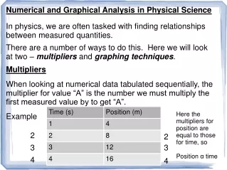
Numerical and Graphical Analysis in Physical Science In physics, we are often tasked with finding relationships between measured quantities. There are a number of ways to do this. Here we will look at two – multipliers and graphing techniques. Multipliers When looking at numerical data tabulated sequentially, the multiplier for value “A” is the number we must multiply the first measured value by to get “A”. Here the multipliers for position are equal to those for time, so Position α time Example 2 2 3 3 4 4
The statement “position α time” is called a “proportionality statement” and is read “position is directly proportional to time”. This means that as time changes, position changes by the same factor (time doubles, position doubles, etc.) Example 2 4 2 9 3 16 4 Power multiplier = Voltage multiplier squared, so ... How is this read? Or P α V2 Power α Voltage2 “Power is directly proportional to the square of Voltage.”
Graphical Analysis A more accurate method of finding this type of relationship is to use graphing. Steps: 1. Plot a scatter graph (that means just the data points for now, no lines yet). Plot the dependent variable on the y-axis unless instructed otherwise. 2. Draw either a straight line of best fit with a ruler, or a curve of best fit freehand. 3. Compare your graph to one of the four common graph types to make a reasonable guess at the relationship between the variables.
Common Graph Types Root Linear Inverse Power
4. For a linear graph, simply determine the value of the slope (called the “constant of proportionality”) and the equation of the line now describes the accurate relationship. 4. For a linear graph, simply determine the value of the slope (called the “constant of proportionality”) and the equation of the line now describes the accurate relationship. 5. For the other three graph types, “Power” is of the form y α xn (n>1), “Root” is of the form and “inverse” is of the form 6. To find the value of n, we can now replot “y” vs. some function of “x” that we choose based on the shape of the first graph. For example, if the first graph looks like a power curve we can plot y vs. x2. 7. Once we have a linear plot, we determine the slope and write the equation of the line. For the power example, if y vs. x2 gives us a straight line, the equation would be y = kx2 + b, where k is slope and b is the y-int.
For the given data set, use graphing techniques to determine the relationship between Force and Frequency.
This graph is clearly not linear, so at least one more graph is required. I'd say it looks like a root graph, so I'll plot a new graph of Frequency vs (in math class you'd call this a graph).
Now we have a linear graph, so we can calculate the slope. = 0.38 So the constant of proportionality is 0.38 Hz/N^0.5. This gives us the equation that describes the relationship between force and frequency: Or, taking the reciprocal of 0.38,