Download
1 / 103
1.04k likes | 1.09k Views
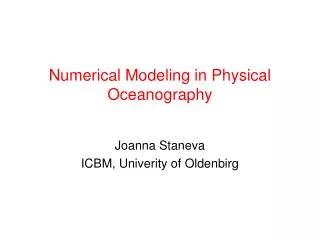
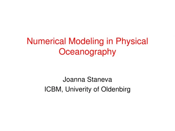
Numerical Modeling in Physical Oceanography. Joanna Staneva ICBM, Univerity of Oldenbirg. What do we study?. Geophysical fluid dynamics. Oceanography Meteorology Climate dynamics. MOTIVATION. Changes in the world ocean are going to be important factors in any global change processes.

E N D
Numerical Modeling in Physical Oceanography Joanna Staneva ICBM, Univerity of Oldenbirg
Geophysical fluid dynamics • Oceanography • Meteorology • Climate dynamics
MOTIVATION • Changes in the world ocean are going to be important factors in any global change processes. • It is difficult to build an „universal'' ocean model that can treat accurately phenomena on all spatial and temporal scales in the various ocean basins. • This is due both to finite computer size and CPU speed, and to an imperfect description of the physical processes, such as turbulence. • Ocean modeling efforts have diversified into different classes,
Free Surface and Rigid Lid Models • In reality, the ocean surface is free to deform under the influence of wind, heating and tidal forces. We find wind-driven waves and surges up to several meters high on its surface. These are typically short-lived, have short spatial scales and fast wave speeds. • In order to avoid the severe limitation on the time step due to the fast gravity waves, one puts a rigid lid on the ocean as this affects the large-scale motions only slightly. The first such model was formulated by Bryan. • This model has been recently reformulated by Killworth et al. to retain the free surface by treating the fast modes separately. Models that treat the fast waves implicitly have been developed by Hurlburt et al.
Fixed Level, Isopycnal, Sigma-Coordinate and Semi-Spectral Models • The models of Bryan and Killworth et al. have all used fixed levels in the vertical -direction, with a variable spacing of the depth levels. • On the other hand, Blumberg and Mellor and Haidvogel et al. have introduced a stretched coordinate - referred to as sigma defined as =z/D, where D is the fluid depth. • In addition Haidvogel et al. have introduced a semi-spectral representation of the vertical dimension (sigma layout) in terms of Chebyshev polynomials (collocation method).
Barotropic vs. Baroclinic Models • Ocean models describe the response of a variable density ocean to atmospheric momentum and heat forcing. This response can very simply be represented in terms of eigenmodes of a linearized system of equations. • The 0-th mode is equivalent to the vertically-averaged component of the motion, also known as the barotropicmode. • The higher modes are called baroclinic modes and are associated with higher order components of the vertical density profile.
Barotropic vs. Baroclinic Models • Many ocean models make the hydrostatic shallow water approximation, in which the pressure depends only on the depth , i.e. it's given by the classic hydrostatic relation dp/dz=z • This relation holds if the horizontal dimensions of the ocean volume under consideration are much larger than the vertical dimension, hence the shallow water designation. • A particular form of the baroclinic models are the so-called reduced gravity models. These are essentially isopycnal models of several deformable layers where the lowest layer has infinite depth and zero velocity.
Barotropic Models Why a barotropic model is interesting and important? • The free surface elevation couples directly to the barotropic mode. (using of satellite altimeter measurements of the free surface elevation). Thus information from altimeters may first enter the ocean model through the barotropic mode, where it represents a direct forcing • The presence of the fast free surface gravity waves. The simple explicit finite-difference schemes treating such waves are subject to severe time step limitations, so that solution of the barotropic mode may lead to large CPU requirements.
Model Equations for a Barotropic Ocean Navier-Stokes equations for incompressible flow on a rotating Earth where:
Boundary conditions closed boundaries in a rectangular geometry
Forcing for Barotropic Models The circulation in a barotropic ocean is generally the result of two kinds of ``forcings'': • the wind stress at the ocean's surface • the source-sink mass flows at the basin boundaries. The source flows could be ocean currents that enter the basin due to wind forcing in an adjacent basin, or enter simply to replace mass driven out by the wind or baroclinic pressure gradients in the model basin. Sink flows have similar origins.
Distribution of Temperature and Salinity Annual mean sea surface temperature
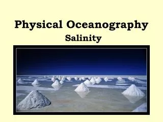
Distribution of Temperature and Salinity Annual mean sea surface salinity
Bottom Topography • Bottom depth is one of the most important parameters for a realistic ocean model. • Bottom depth is derived from acoustic soundings from a ship. • Very high resolution (approaching 1 km) bottom topography is generally not available in the public domain. • The best resolution public domain topography thus far is the gridded ETOP5 at NCAR, which contains 5 min resolution of Earth's topography. • Another topographic data set is the DBDB-5 (Digital Bathymetry Data Base at 5 min intervals), developed by the U.S. Naval Oceanographic
On finite differencing • Typical equation in Oceanography and Geophysical Fluid Dynamics (GFD) • On finite differences • Finite difference form of equations • Higher order schemes • Time evolution • More complex models and grid arrangements • PROBLEMS!
On finite differencing • Typical equation in Oceanography and Geophysical Fluid Dynamics (GFD) • On finite differences • Finite difference form of equations • Higher order schemes • Time evolution • More complex models and grid arrangements • PROBLEMS!
Typical equations in Oceanography • Equations • Boundary conditions or
On finite differencing • Typical equation in Oceanography and Geophysical Fluid Dynamics (GFD) • On finite differences • Finite difference form of equations • Higher order schemes • Time evolution • More complex models and grid arrangements • PROBLEMS!
Taylor expansion For the first order derivative which is correct to order:
More accurate scheme For the first order derivative which is correct to order:
Second order derivative (1)+(2) and rearranging: which is correct to order:
Large variety of scales Parameterizations are important in geophysical fluid dynamics
Timescales • Atmospheric low pressures: 10 days • Seasonal/annual cycles: 0.1-1 years • Ocean eddies: 0.1-1 year • El Nino: 2-5 years. • North Atlantic Oscillation: 5-50 years. • Turnovertime of atmophere: 10 years. • Anthropogenic forced climate change: 100 years. • Turnover time of the ocean: 4.000 years. • Glacial-interglacial timescales: 10.000-200.000 years.
Timescales • Atmospheric low pressures: 10 days • Seasonal/annual cycles: 0.1-1 years • Ocean eddies: 0.1-1 year • El Nino: 2-5 years. • North Atlantic Oscillation: 5-50 years. • Turnovertime of atmophere: 10 years. • Anthropogenic forced climate change: 100 years. • Turnover time of the ocean: 4.000 years. • Glacial-interglacial timescales: 10.000-200.000 years.
Timescales • Atmospheric low pressures: 10 days • Seasonal/annual cycles: 0.1-1 years • Ocean eddies: 0.1-1 year • El Nino: 2-5 years. • North Atlantic Oscillation: 5-50 years. • Turnovertime of atmophere: 10 years. • Anthropogenic forced climate change: 100 years. • Turnover time of the ocean: 4.000 years. • Glacial-interglacial timescales: 10.000-200.000 years.
Timescales • Atmospheric low pressures: 10 days • Seasonal/annual cycles: 0.1-1 years • Ocean eddies: 0.1-1 year • El Nino: 2-5 years. • North Atlantic Oscillation: 5-50 years. • Turnovertime of atmophere: 10 years. • Anthropogenic forced climate change: 100 years. • Turnover time of the ocean: 4.000 years. • Glacial-interglacial timescales: 10.000-200.000 years.