Linear Separability
3. 3. 3. x 2. x 2. x 2. 2. 2. 2. 1. 1. 1. -3. -3. -3. -2. -2. -2. -1. -1. -1. 1. 1. 1. 2. 2. 2. 3. 3. 3. x 1. x 1. x 1. -1. -1. -1. -2. -2. -2. -3. -3. -3. Linear Separability. Input space in the two-dimensional case (n = 2):. 1. 1. 1. 0. 0. 0.

Linear Separability
E N D
Presentation Transcript
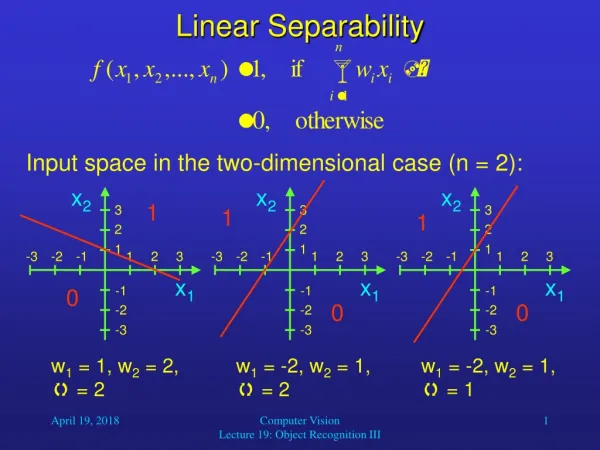
3 3 3 x2 x2 x2 2 2 2 1 1 1 -3 -3 -3 -2 -2 -2 -1 -1 -1 1 1 1 2 2 2 3 3 3 x1 x1 x1 -1 -1 -1 -2 -2 -2 -3 -3 -3 Linear Separability Input space in the two-dimensional case (n = 2): 1 1 1 0 0 0 w1 = 1, w2 = 2, = 2 w1 = -2, w2 = 1, = 2 w1 = -2, w2 = 1, = 1 Computer Vision Lecture 19: Object Recognition III
Linear Separability • So by varying the weights and the threshold, we can realize any linear separation of the input space into a region that yields output 1, and another region that yields output 0. • As we have seen, a two-dimensional input space can be divided by any straight line. • A three-dimensional input space can be divided by any two-dimensional plane. • In general, an n-dimensional input space can be divided by an (n-1)-dimensional plane or hyperplane. • Of course, for n > 3 this is hard to visualize. Computer Vision Lecture 19: Object Recognition III
Capabilities of Threshold Neurons • What do we do if we need a more complex function? • We can combine multiple artificial neurons to form networks with increased capabilities. • For example, we can build a two-layer network with any number of neurons in the first layer giving input to a single neuron in the second layer. • The neuron in the second layer could, for example, implement an AND function. Computer Vision Lecture 19: Object Recognition III
x1 x1 x1 x2 x2 x2 xi . . . Capabilities of Threshold Neurons • What kind of function can such a network realize? Computer Vision Lecture 19: Object Recognition III
2nd comp. 1st comp. Capabilities of Threshold Neurons • Assume that the dotted lines in the diagram represent the input-dividing lines implemented by the neurons in the first layer: Then, for example, the second-layer neuron could output 1 if the input is within a polygon, and 0 otherwise. Computer Vision Lecture 19: Object Recognition III
Capabilities of Threshold Neurons • However, we still may want to implement functions that are more complex than that. • An obvious idea is to extend our network even further. • Let us build a network that has three layers, with arbitrary numbers of neurons in the first and second layers and one neuron in the third layer. • The first and second layers are completely connected, that is, each neuron in the first layer sends its output to every neuron in the second layer. Computer Vision Lecture 19: Object Recognition III
x1 x1 x1 x2 x2 x2 oi . . . . . . Capabilities of Threshold Neurons • What type of function can a three-layer network realize? Computer Vision Lecture 19: Object Recognition III
2nd comp. 1st comp. Capabilities of Threshold Neurons • Assume that the polygons in the diagram indicate the input regions for which each of the second-layer neurons yields output 1: Then, for example, the third-layer neuron could output 1 if the input is within any of the polygons, and 0 otherwise. Computer Vision Lecture 19: Object Recognition III
Capabilities of Threshold Neurons Computer Vision Lecture 19: Object Recognition III
Capabilities of Threshold Neurons • The more neurons there are in the first layer, the more vertices can the polygons have. • With a sufficient number of first-layer neurons, the polygons can approximate any given shape. • The more neurons there are in the second layer, the more of these polygons can be combined to form the output function of the network. • With a sufficient number of neurons and appropriate weight vectors wi, a three-layer network of threshold neurons can realize any (!) function Rn {0, 1}. Computer Vision Lecture 19: Object Recognition III
Terminology • Usually, we draw neural networks in such a way that the input enters at the bottom and the output is generated at the top. • Arrows indicate the direction of data flow. • The first layer, termed input layer, just contains the input vector and does not perform any computations. • The second layer, termed hidden layer, receives input from the input layer and sends its output to the output layer. • After applying their activation function, the neurons in the output layer contain the output vector. Computer Vision Lecture 19: Object Recognition III
Terminology output vector • Example: Network function f: R3 {0, 1}2 output layer hidden layer input layer input vector Computer Vision Lecture 19: Object Recognition III
General Network Structure Computer Vision Lecture 19: Object Recognition III
Feedback-Based Weight Adaptation • Feedback from environment (possibly teacher) is used to improve the system’s performance • Synaptic weights are modified to reduce the system’s error in computing a desired function • For example, if increasing a specific weight increases error, then the weight is decreased • Small adaptation steps are needed to find optimal set of weights • Learning rate can vary during learning process • Typical for supervised learning Computer Vision Lecture 19: Object Recognition III
Network Training • Basic idea: Define error function tomeasure deviation of network output from desired output across all training exemplars. • As the weights of the network completely determine the function computed by it, this error is a function of all weights. • We need to find those weights that minimize the error. • An efficient way of doing this is based on the technique of gradient descent. Computer Vision Lecture 19: Object Recognition III
Gradient Descent • Gradient descent is a very common technique to find the absolute minimum of a function. • It is especially useful for high-dimensional functions. • We will use it to iteratively minimizes the network’s (or neuron’s) error by finding the gradient of the error surface in weight-space and adjusting the weights in the opposite direction. Computer Vision Lecture 19: Object Recognition III
f(x) slope: f’(x0) x0 x1 = x0 - f’(x0) x Gradient Descent • Gradient-descent example: Finding the absolute minimum of a one-dimensional error function f(x): Repeat this iteratively until for some xi, f’(xi) is sufficiently close to 0. Computer Vision Lecture 19: Object Recognition III
Gradient Descent • Gradients of two-dimensional functions: The two-dimensional function in the left diagram is represented by contour lines in the right diagram, where arrows indicate the gradient of the function at different locations. Obviously, the gradient is always pointing in the direction of the steepest increase of the function. In order to find the function’s minimum, we should always move against the gradient. Computer Vision Lecture 19: Object Recognition III
Multilayer Networks • The backpropagation algorithm was popularized by Rumelhart, Hinton, and Williams (1986). • This algorithm solved the “credit assignment” problem, i.e., crediting or blaming individual neurons across layers for particular outputs. • The error at the output layer is propagated backwards to units at lower layers, so that the weights of all neurons can be adapted appropriately. Computer Vision Lecture 19: Object Recognition III
Backpropagation Learning • AlgorithmBackpropagation; • Start with randomly chosen weights; • while MSE is above desired threshold and computational bounds are not exceeded, do • for each input pattern xp, 1 p P, • Compute hidden node inputs; • Compute hidden node outputs; • Compute inputs to the output nodes; • Compute the network outputs; • Compute the error between output and desired output; • Modify the weights between hidden and output nodes; • Modify the weights between input and hidden nodes; • end-for • end-while. Computer Vision Lecture 19: Object Recognition III
Supervised Function Approximation • There is a tradeoff between a network’s ability to precisely learn the given exemplars and its ability to generalize (i.e., inter- and extrapolate). • This problem is similar to fitting a function to a given set of data points. • Let us assume that you want to find a fitting function f:RR for a set of three data points. • You try to do this with polynomials of degree one (a straight line), two, and nine. Computer Vision Lecture 19: Object Recognition III
deg. 2 f(x) deg. 1 deg. 9 x Supervised Function Approximation • Obviously, the polynomial of degree 2 provides the most plausible fit. Computer Vision Lecture 19: Object Recognition III
Supervised Function Approximation • The same principle applies to ANNs: • If an ANN has too few neurons, it may not have enough degrees of freedom to precisely approximate the desired function. • If an ANN has too many neurons, it will learn the exemplars perfectly, but its additional degrees of freedom may cause it to show implausible behavior for untrained inputs; it then presents poor ability of generalization. • Unfortunately, there are no known equations that could tell you the optimal size of your network for a given application; there are only heuristics. Computer Vision Lecture 19: Object Recognition III
Reducing Overfitting with Dropout • During each training step, we “turn off” a randomly chosen subset of 50% of the hidden-layer neurons, i.e., we set their output to zero. • During testing, we once again use all neurons but reduce their outputs by 50% to compensate for the increased number of inputs to each unit. • By doing this, we prevent each neuron from relying on the output of any particular other neuron in the network. • It can be argued that in this way we train an astronomical number of decoupled sub-networks, whose expertise is combined when using all neurons again. • Due to the changing composition of sub-networks it is much more difficult to overfit any of them. Computer Vision Lecture 19: Object Recognition III
Reducing Overfitting with Dropout Computer Vision Lecture 19: Object Recognition III