Download
1 / 26

E N D
Representation of Waves 1/2 Any periodic motion of a fluid can be decomposed by Fourier analysis into a superposition of sinusoidal oscillations with different frequencies and wavelengths . A simple wave is any one of these components. When the oscillation amplitude is small, the waveform is generally sinusoidal and there is only one component. This is the situation we will consider. Any oscillating quantity, say density n, can be represented by n = ñexp(i(k.r-t)) (3.1-1) ñ is the constant amplitude, k is the propagation vector. For motion only in the x direction n = ñexp(i(kx-t)) (3.1-2) By convention, the exponential notation means that the real part of the expression is taken as the measurable quantity. Let us choose ñ to be real. We shall see that this corresponds to a choice of the origins of x and t. Re(n) = ñcos(kx-t) (3.1-3) A point of constant phase on the wave moves so that d((kx-t)/dt = 0, so dx/dt = /k = vp (3.1-4) where vp is the so-called phase velocity. If /k > 0 the wave moves to the right (positive x) and if /k < 0 the wave moves to the left.
Representation of Waves 2/2 E = Êcos((kx-t+) (3.1-5) or E = Êexp(i(kx-t+)) (3.1-6) where Ê is a real, constant vector. It is customary to incorporate the phase information into Ê by allowing Ê to be complex. Thus, we can write E = Êexp(i)exp(i(kx-t)) = Ëexp(i(kx-t)) (3.1-7) where Ë = E = Êexp(i) and Re(Ë) = Êcos, and Im(Ë) = Êsin (3.1-8) so tan = Im(Ë)/Re(Ë) (3.1-9) From now on we will assume all amplitudes of vectors are complex and drop the awkward notation with the umlaut! Any oscillating quantity will be written as g = g1exp(i(k.r-t)) (3.1-10) so that g1 can stand for either the complex amplitude or the whole expression. (3.1-10). There will be no confusion because in linear wave theory (which is what we will be looking at) the same exponential factor will occur on both sides of the equation and will cancel out.
Worked Example Q. The oscillating density n1 and potential 1 in a drift wave are related by n1/n0 = (e1/ kBTe)(* + ia)/( + ia) (3.1-11) where it is only necessary to know that all other symbols (except i) stand for real, positive constants. a) Find an expression for the phase of 1 with respect to n1 (for simplicity assume that n1 is real). b) If < * does 1 lead or lag n1? A. From (3.1-11) solve for 1 ((kBTe)/e).(* + a2 +ia(* - )/(*2 + a2).(n1/n0) (3.1-12) Im(1)/Re((1) = a((* - )/(* + a2) = tan (3.1-13) a) Hence = tan-1(a((* - )/(* + a2)) (3.1-14) b) For < *, > 0. n1 = n0 exp(i(kx-t)) while 1 = Aexp(i(kx-t+)) where A is a positive constant. Let the phase of n1 be 0 at x0, t0 i.e. (kx0,-t0) = 0. If and k are positive and x0 is fixed, then the phase of 1 atx0 is 0when (kx0-t+) = 0 at t > t0. Hence 1 lags n1 in time. If t0 is fixed, (kx-t0+) = 0 at x < x0, so 1 lags n1 in space as well.
Group Velocity To illustrate this we consider a modulated wave formed by adding (“beating”) two waves of nearly equal frequencies. Let these waves be; E1 = E0cos(k+k)x – (+)t (3.2-1) E2 = E0cos(k-k)x – (-)t E1 and E2 differ in frequency by 2. Since each wave must have a phase velocity of /k appropriate to the medium in which they propagate one must allow for a difference 2k in the propagation constant. The superposition of the waves leads to; E1+ E2 = 2E0 cos(k)x – ()tcos(kx-t) (3.2-2) which is a modulated wave. The envelope of the wave given by cos(k)x – ()t is what carries the information . It travels at a velocity of /k. Taking the limit as the increments tend to zero we define the group velocity to be vg = d /dk (3.2-3) It is this quantity that cannot exceed c.
Plasma Oscillations1/2 • If the electrons in a plasma are displaced form a uniform background of ions, electric fields will be built up in such a direction as to restore the neutrality of the plasma by pulling the electrons back to their original positions. Because of their inertia the electrons will overshoot and oscillate around their equilibrium positions with a frequency known as the plasma frequency. The oscillation is so fast that the massive ions do not have time to respond to the oscillating field and so can be considered as fixed. • To derive this frequency we assume; • 1) no magnetic field • 2) no thermal motion (kBT = 0) • 3) ions are fixed in space in a unform distribution • 4) the plasma is infinite in extent • 5) electron motions occur only in the x direction • As a consequence of assumption 5) • = xu∂/∂x, E = Exu ,x E = 0 hence E = -1 (3.3.1-1) • where xu is a unit vector in the x direction. There is no fluctuating magnetic field. This is an electrostatic oscillation. Now the electron equation of motion is • mne∂ ve/∂t + (ve. )ve = - ene E (3.3.1-2) • and the equation of continuity is • ∂ne/∂t + .(ne ve) = 0 (3.3.1-3) • The only Maxwell’s equation we need is the Poisson’s equation (this case is an exception to the general • rule in lecture 2 that the Poisson’s equation cannot be used to find E); • 0.E= xu . xu ∂E/∂x = e(ni – ne) (3.3.1-4) • Linearise these equations. This means that we set • ne = n0 + n1 ve = ve0 + ve1 E = E0 +E1 (3.3.1-5)
Plasma Oscillations 2/2 The deviations (perturbations, suffix 1 quantities) from the equilibrium (suffix 0 quantities) are small so that only first order quantities are retained in the analysis. The equilibrium quantities express the state of the plasma in the absence of the oscillation. Note nio = neo, from Poisson’s equation and ni1 from the assumption of fixed ions. n0 = ve0 = E0 = 0 (3.3.1-6) ∂n0/∂t = ∂ve0 /∂t = ∂E0/∂t (3.3.1-2) becomes m∂ ve1∂t = - eE1 (3.3.1-7) 3.3.1-3) becomes ∂n1/∂t + n0. ve1 = 0 (3.3.1-8) and (3.3.1-4) becomes 0.E1 = -e n1 (3.3.1-9) The oscillating quantities are assumed to behave sinusoidally i.e. n1 = n1exp(i(kx-t) ve1 = ve1exp(i(kx-t)xuE1 = E1exp(i(kx-t)xu (3.3.1-10) The time derivative can therefore be replaced by -i and the gradient by ik xu The 3 equations (3.3.1-7 to 9) become - imve1 = - eE1 (3.3.1-11) - in1 + ik n0 ve1 = 0 (3.3.1-12) 0ikE1 = - en1 (3.3.1-13) Eliminating n1 and E1 we have (3.3.1-11) - imve1 = -e.(-e/(0ik)).(-(ik n0 ve1)/(-i) = -in0 e2/(0)ve1 (3.3.1-14) so that if ve1 is not equal to zero then 2 = n0 e2/(m0) (3.3.1-15) and this is the plasma frequency p, a fundamental plasma quantity.
Electron Plasma Waves There is another effect that causes plasma oscillations to propagate and that is thermal motion. Electron s treaming into adjacent layers of plasma with their thermal velocities will carry information about what is happening in the oscillating region. The plasma oscillation can then properly be called a plasma wave. This effect can be included by adding a term - pe to the electron equation of motion (3.3.1-2). From lecture 2, the equation of state is pe /pe = n/n (3.3.2-1) where is the ratio of specific heats at constant pressure and constant volume (= Cp/Cv) = (2 + N)/N where N is the number of degrees of freedom involved. In the present case, we consider one dimensional motion (N = 1) so that = 3 and ; pe = 3 pen/n = 3kBTe(n0 + n1) = 3kBTe xu∂n1/∂x (3.3.2-2) The linearised equation of motion for electrons becomes mn0∂v1/∂t = - en0E1 - 3kBTe∂n1/∂x (3.3.2-3) with the assumptions of oscillating perturbations of (3.3.1-10) this becomes -imn0v1= - en0E1 - 3kBTeikn1 (3.3.2-4) Using the expressions (3.3.1-12) and (3.3.1-13) for E1 andn1 we have imn0v1 =en0(-e/(ik//0) + 3kBT/m.k2v1 (3.3.2-5) which gives (for non-zero v1) 2 = p2 + 3/2k2vth2 (3.3.2-6)
Sound Waves in Air • As an introduction to ion waves in a plasma let us briefly review the theory of sound waves in air. • Neglecting viscosity we can write the Navier-Stokes equation which describes these waves as; • ∂v/∂t + v.v = - p = - (p/)(3.3.3-1) • The equation of continuity is • ∂/∂t + .(v0) = 0 (3.3.3-2) • Linearising these equations around a stationary equilibrium with uniform p0 and 0 gives • -i0v1= -(p0/0)ik/1 (3.3.3-3) • -i1 +ik. v1 = 0 (3.3.3-4) • where we have (as usual) taken the wave dependence of the perturbation of the form exp(i(k.r - t)). • For a plane wave with k = kxu and v = vxu we find on eliminating /1 • -i0v1 = -(p0/0)ik(0ik. v1/( i)) (3.3.3-5) • which for non-zero v1 gives • 2 = (p0/0) = (kBT/M) = cs2 (3.3.3-6) • where cs is the speed of sound in a neutral gas. The wave propagates from one layer to the next by collisions among air molecules.
Ion Acoustic Waves 1/2 In a plasma there is an analogous phenomenon, the ion acoustic wave. In the absence of collisions, ordinary acoustic waves should not occur. However, ions can still transmit vibrations to each other because of their charge and acoustic waves occur through the intermediary of an electric field. Since the motion of the massive ions will be involved, the oscillations will be low frequency and we can use the plasma approximation of lecture 2. The ion fluid equation in the absence of magnetic field is Mini∂vi/∂t + vi.vi = eniE -p = - e - i kBTini (3.3.3-7) where we have assumed E = - and used the equation of state. Linearising and assuming plane waves, we have -iMin0vi1= - eni0ik1 -i kBTiiikn1 (3.3.3-8) For the electrons we assume no inertia (i.e. me very small), and therefore the electron equation of motion gives the balance of forces -e∂/∂x = -ikBTe/(mene)∂ne/∂x (3.3.3-9) which gives ne = ne0meexp(e/(kBTe) (3.3.3-10) and in linearised form ne1 = ne0(e1/(kBTe) (3.3.3-11) where 0 is assumed to be zero (E0 = 0), and for quasineutrality, this perturbation in electron density is the same as that for the perturbation in ion density so that ne1 = ni1.The linearised equation of continuity for ions is in1 = n0ikvi1 (3.3.3-12) Eliminating n1 and 1 from (3.3.3-8 , 11 and 12) we have, for non-zero vi1 2 = k2(kBTe/Mi+ i kBTi/Mi) (3.3.3-13)
Ion Acoustic Waves 2/2 In deriving the ion waves we have assumed ni = ne while allowing E to be finite. To see what error is involved we now allow these densities to be differentand use the linearised Poisson’s equation: 0.E1 = 0k21= e(ni1 – ne1) (3.3.3-15) Using ne1 (= ne0(e1/(kBTe)) from (3.3.3-11) in (3.3.3-15) we obtain 01(k2 + ne0 e2/(0kBTe)) = eni1 (3.3.3-16) 01(k2 D2+ 1) = eni1D2 (3.3.3-17) The ion density perturbation is given by the linearised ion continuity equation (3.3.3-12), which, together with (3.3.3-17), if inserted into the linearised ion equation of motion (3.3.3-8) gives iMin0vi1= (en0 ik/0.eD2/(1 + k2 D2) + i kBTiiik) n0kvi1/() (3.3.3-18) so that for non-zero vi1 /k = vs = (kBTe/Mi/(1 + k2 D2) + i kBTi/Mi)0.5 (3.3.3-19) This is the same as obtained previously (3.3.3-14) except for the factor 1 + k2 D2. Since D is small in most situations, the plasma approximation used to derive the ion acoustic wave dispersion relation (3.3.3-14) is valid for all except the shortest wavelengths.If we consider k2 D2 >> 1 (and for simplicity kBTi = 0) then from (3.3.3-19) 2 = k2n0e2/(0. Mi k2)= n0e2/(0Mi) = p2 (3.3.3-20) where p2 is the ion plasma frequency.
Waves in a Magnetised Plasma Parallel and perpendicular refer to the direction of k with respect to the undisturbed magnetic field B0. Longitudinal and transverse refer to the direction of k with respect to the oscillating electric field E1. If the oscillating magnetic field B1 is zero, then the wave is electrostatic, otherwise it is electromagnetic. The last two sets of terms are related by the Maxwell equation; xE1 = -∂B1/∂t (3.4-1) or kx E1 = -B1 (3.4-2) If the wave is longitudinal then kx E1 vanishes and the wave is electrostatic. If the wave is transverse, and B1 is finite, then the wave is electromagnetic. If k is at an arbitrary angle to B0.or E1 is finite then one would have a mixture of the principal modes presented here.
Electrostatic Electron Oscillations Perpendicular to B0 We start with the high frequency, electrostatic, electron oscillations propagating at right angles to B. We assume that the ions are too massive to move at the frequencies involved and form a uniform background of positive charge. We shall also neglect thermal motions and set kBTe = 0. The equilibrium plasma has constant and uniform density, n0, and magnetic field B0, and magnetic field B0 and zero electric field E0. The motion of electrons is then governed by the linearised equations of motion, continuity and Poisson’s equation: m∂ve1/∂t = e(E1 + ve1xB0) (3.4.1-1) ∂ ne1/∂t + n0,.(ve1) = 0 (3.4.1-2) 0.E1 = - ene1 (3.4.1-3) We consider longitudinal waves so that kE1. Without loss of generality we can choose the x-axis to lie along k and E1 andB0 to lie along the z axis.Thus ky = kz = Ey = Ez = 0, k = kxxuand E = Exxu Separating (3.4.1-1) into components and assuming the sinusoidal wave dependences for the perturbations: - ive1x = - e(E1x + ve1yxB0) (3.4.1-4) - ive1y = eve1xxB0 (3.4.1-5) - ive1z = 0 (3.4.1-6) Substituting for ve1y from(3.4.1-5) in (3.4.1-4) gives ve1x = eE1x/(im)/(1- c2/2) (3.4.1-7) Note that this becomes infinite at the cyclotron resonance = c This is to be expected since the electric fieldchanges sign with ve1x so that the electrons are continuously accelerated by it. From the linearised equation of continuity (3.4.1-2), ne1 = n0,kx.ve1x/ (3.4.1-8) Linearising Poisson’s equation (3.4.1-3) and using the expressions for ve1x andne1 gives, for non-zero E1x 2 = c2 + p2 = h2 (3.4.1-9) The frequency his the upper hybrid frequency.
Electrostatic Ion Waves Perpendicular to B0 1/2 It is tempting to set k.B0 exactly equal to zero when k is perpendicular to B0.This would lead to a result which although mathematically correct does not describe what happens in real plasmas. Instead we shall assume that k is almost perpendicular to B0. We assume, as usual, an infinite plasma in equilibrium with n0 and B0 constant and uniform and v0= E0 = 0. For simplicity we take Ti = 0. We will not miss any important effects as we know that acoustic waves still exist for Ti = 0. We also assume electrostatic waves with kxE = 0 so that E = -. k and E are in the x-z plane at an angle to B0 (along the z axis) i.e. the angle of k and E with respect to the x axis is /2 - which is small. As far as the ion motion is concerned we may take = ikxu and E =E1xu. For the electrons it makes a great deal of difference whether /2 - is zero, or small but finite. The electrons have such small Larmor orbits (rotation around the magnetic field), that they cannot move in the x direction to preserve charge neutrality. The E field does make them drift (ExB drift) back and forth in the y direction. If is not exactly equal to /2, the electrons can move in the z direction (along B0) to carry charge from negative to positive regions in the wave and carry out Debye shielding. The ions cannot do this because of their inertia which prevents them from moving long distances in a wave period. That is why we neglect kz for ions. The following treatment is OK for small angles /2 - > (m/M)0.5 (the ratio of the ion and electron velocities for equal particle energies) For /2 - < (m/M)0.5. the treatment of the next section 4.3 is appropriate. For the linearised, ion equation of motion we have Mi∂vi1/∂t = - e1 + e vi1xB0 (3.4.2-1)
Electrostatic Ion Waves Perpendicular to B0 2/2 • Assuming plane waves propagating in the x direction (kx = k) and separating this equation into its x and y components, • -iMivi1x = - eik1 + evi1yB0 • (3.4.2-2) • -iMivi1y = -evi1xB0 • Solving for vi1x we have; • vi1x =ek1/(Mi) (1- c2/2)-1 (3.4.2-3) • where c= eB0 /Mi is the ion cyclotron frequency.The ion equation of continuity yields • ni1 = n0,kvi1x/ (3.4.2-4) • Assuming the electrons can move along B0 because of the finiteness of /2 - we can use the Boltzmann relation for electrons • ne1 = ne0(e1/(kBTe) (3.4.2-5) • The plasma approximation ni = ne now closes the system of equations so that we are left with 2 equations for 1 and vi1x. Eliminating 1 gives for non-zero vi1x • 2 = c2 + k2vs2 (3.4.2-6) • where vs is the sound speed in the plasma (see (3.3.3-19)). This is the dispersion relation for ion cyclotron (electrostatic) waves.
Lower Hybrid Frequency • We now consider what happens for the case /2 = (in fact /2 - < (m/M)0.5. Instead of obeying Boltzmann’s relation the electrons will obey the full equation of motion. If we keep the electron mass finite this equation is non-trivial even if we assume that Te = 0 and so we drop the pe term. The ion equation of motion is as for (3.4.2-3) i.e. • vi1x =ek1/(Mi) (1- c2/2)-1 (3.4.3-1) • In a manner similar to the analysis for the ion equation of motion (consider (3.4.2-2) and change e to – e, M to m, and c to - c with Te = 0) • ve1x =ek1/(me) (1- c2/2)-1 (3.4.3-2) • Now from the equations of continuity • ni1 = n0,kvi1/ (3.4.3-3) • ne1 = n0,kve1/ (3.4.3-4) • The plasma approximation ni = ne then requires vi1 = ve1 so that (3.4.3-1) and • (3.4.2-3) give • = (c2c2)0.5 = l (3.4.3-5) • This is the lower hybrid frequency. If we had used Poisson’s equation instead of the plasma approximation • we would have obtained • 1/l2 = 1/(cc) + 1/p2 (3.4.3-6) • In low density plasma the last term actually dominates. The plasma approximation is not valid at such • high frequencies. Lower hybrid oscillations can be observed only when is very close to /2.
Electromagnetic Waves with B0 = 0 1/2 • Next in the order of complexity come waves with B1 not equal to zero. These are transverse electro- • magnetic waves-light waves or radio waves traveling through a plasma. We begin with a brief review of • such waves in a vacuum. The relevant Maxwell equations are: • xE1 = ∂B1∂t (3.4.4-1) • c2xB1 =∂E1∂t (3.4.4-2) • since in a vacuum j = 0 and c2 =1/0 0. Taking the curl of (3.3.4.4-2) and substituting the time derivative • of (3.3.4.3-1) gives, • c2x(xB1) = xE1 = ∂2B1∂t2 (3.4.4-3) • Assuming plane waves varying as exp (i(kx-t)) we have • 2 B1 = - c2(kx(kxB1) = - c2(((k. B1)k - k2B1) (3.4.4-4) • Now since k. B1 = -i.B1 = 0 the result is • 2 = k2 c2 (3.4.4-5) • and c is the phase velocity of the waves. • Now for the plasma case, (3.4.4-1) remains the same but we have to add to (3.4.4-2) the term j/0, to • account for currents due to the first order charged particle motions so that • c2xB1 =∂E1/∂t + j1/0 (3.4.4-6) • The time derivative of this is • c2x∂B1 /∂t=∂2E1/∂t 2+ (∂j1/∂t)/0 (3.4.4-7) • Taking the curl of (3.4.4-1) gives • x(xE1 )= (. E1) - 2E1 = -x∂B1∂t (3.4.4-8) • Using x∂B1∂t from (3.4.4-7) and assuming a wave dependence exp(i(k.r - t)) • -k(k.E1) + k2E1 =2/c2E1 + i/(0 c2)j1 (3.4.4-9)
Electromagnetic Waves with B0 = 0 2/2 • By transverse wave we mean k.E1 = 0so that • (2 - c2 k2)E1 = - i/(0)j1 (3.4.4-10) • If we consider light waves or microwaves, these will be of such high frequency that the ions can be • considered as fixed. The current j1 then comes entirely from the electrons • j1 = - n0eve1 (3.4.4-11) • From the linearised equation of motion for the electrons we have • me∂ve/∂t = - eE(3.4.4-12) • so that ve1 = eE1/(ime) (3.4.4-13) • and for non-zero E1 • 2= pe2 +c2k2 (3.4.4-14) • This is the dispersion relation for electromagnetic waves propagating in a plasma with no steady • magnetic field. The vacuum dispersion relation is modified by the term pe2 reminiscent of plasma • oscillations. The phase velocity vp is greater than c, but the group velocity vg is c2/vp i.e. less than c. • This dispersion relation exhibits a phenomenon known as cutoff. If one sends a microwave beam of a • given frequency through a plasma, the wavelength 2/k in the plasma will take on the value prescribed • by the dispersion relation (3.4.4-14). As the plasma density, and hence pe increases, k will necessarily • decrease. At some density (the cutoff density), k will be zero. For densities larger than this the dispersion relation cannot be satisfied for real k and hence the wave cannot propagate. The critical density (nc) (such that = pe) is • nc = me02/e2 (3.4.4-15) • If n is too large or too small, an electromagnetic wave cannot pass beyond this point in the plasma. • When this happens, k is imaginary ck = i pe 2 - 20.5 and because the spatial dependence of the wave • is exp(ikx), it will be exponentially attenuated as exp(-x/) where the characteristic attenuation length • or skin depth is • = k-1 = c/( pe 2 - 20.5) (3.4.4-16)
Electromagnetic Waves B0: Ordinary Wave (E1B0) • For kE1 transverse waves, and perpendicular propagation kB0 , there are still 2 choices: E1B0 or E1B0.Here we treat the first case (ordinary wave), and then we treat the other case (extraordinary wave). • Ordinary Wave • If E1B0 we may take B0 = B0zu, E1= E1zu, and k = kxu. The wave equation is still given by (3.4.4-10) • (2 - c2 k2)E1 = - i/(0)j1 = in0e/(0)ve1 (3.4.5-1) • where we have used the expression for j1 (3.4.4-11). Since E1= E1zu we need only the component ve1z which is given by the electron equation of motion • me∂vez/∂t = - eEz (3.4.5-2) • Since this is the same equation as for the case B0= 0, the result is the same (3.4.4-14); • 2= pe2 + c2k2 (3.4.5-3)
Electromagnetic Waves B0:Extraordinary Wave (E1B0) 1/2 • As above we take B0 = B0zu. If E1B0 electron motion will be affected by the magnetic field and the • dispersion relation will be altered. To treat this case we allow E1 to have both x and y components • E1 = E1xxu + E1yyu (3.4.5-4) • The linearised equation of motion for the electrons is • me∂ve1/∂t = - e(E1 + e ve1xB0) (3.4.5-5) • Only the x and y components are non-trivial. They are; • ve1x = -ie/(me)(E1x+ v1yB0) • (3.4.5-6) • ve1y = -ie/(me)(E1y- v1xB0) • Solve for v1x and v1y gives • ve1x = e/(me)(-iE1x- c/E1y)(1- (c/)2)-1 • (3.4.5-7) • ve1y = e/(me)(-iE1y+ c/ E1x)(1- (c/)2)-1 • The wave equation is (3.4.4-9) where we must now retain k.E1 = kE1x to obtain • (2 - c2k2)E1 + c2kE1xk = - i/(0)j1 = in0e/(0)ve1 (3.4.5-8)
Electromagnetic Waves B0:Extraordinary Wave (E1B0) 2/2 Separating this into the 2 components (x and y) and using the expressions (3.4.5-6) 2E1x = -in0e/(0)e/(me)(iE1x+ c/E1y)(1- (c/)2)-1 (3.4.5-9) (2 - c2k2)E1y = -in0e/(0)e/(me)(iE1y- c/E1x)(1- (c/)2)-1 Introducing the expression for p these equations can be written as (2(1- (c/)2) - p2)E1x + i p2c/ E1y = 0 (3.4.5-10) (2- c2k2)(1- (c/)2) - p2)E1y - i p2c/E1x = 0 The condition that these simultaneous equations for E1x and E1y are compatible is that the determinant of the matrix multiplier is zero, and this condition gives the dispersion relation, which after some algebra can be written c2k2/2 = c2/vp2 = 1 - (p/)2(2 - p2)/(2 - h2) (3.4.5-11)
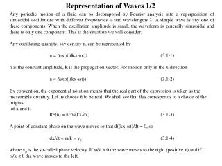
Cutoffs and Resonances for the Extraordinary Wave • The dispersion relation for the extraordinary wave is considerably more complicated than any we have • met up with. To analyse it it is useful to define the terms cutoff and resonance. A cutoff occurs when • the index of refraction (c/vp = ck/) goes to zero i.e. when the wavelength becomes infinite. A • resonance occurs when the index of refraction becomes infinite i.e. the wavelength goes to zero (k goes to infinity). A wave is generally reflected at a cutoff and absorbed at a resonance. • The cutoffs and resonances of the extraordinary wave can be found from the dispersion relation. • The resonances are given by • h2 = p2 + c2 = 2 (3.4.5-12) • which is recognized as the dispersion relation for electrostatic waves propagating across B0. As a wave • of a given frequency approaches the resonance point both its phase and group velocity approach zero • and the wave energy is converted into upper hybrid oscillations. The extraordinary wave is partly • electromagnetic and partly electrostatic. At the resonance it loses its electromagnetic character and • becomes an electrostatic oscillation. • The cutoffs are given by (algebra!) • (1 - (p/)2)2 = (c/)2 (3.4.5-13) • 2 ± c -p2) = 0 (3.4.5-14) • The two roots of this equation are called the left-hand L and the right-hand R cutoffs. • R = 0.5(c + ((c2 + 4p2)0.5) (3.4.5-15) • L =0.5(-c + ((c2 + 4p2) 0.5) (3.4.5-16)
v2/c2 ` 1 0 L p R h
Electromagnetic Waves Parallel to B0 We take B0 = B0zu, E so k lie along the z axis, and allow E to have both x and y components. k = kzu and E1 = E1xxu + E1yyu (3.4.6-1) The wave equation for the extraordinary wave (3.3.4.5-8) can still be used if we simply change k from kxu to kzu (2 - c2k2)E1x = p2/2 (E1x-ic/E1y)(1- (c/)2)-1 (3.4.6-2) (2 - c2k2)E1y = p2/2(E1y+ ic/E1x)(1- (c/)2)-1 This leads to the coupled equations for E1x and E1y (2 - c2k2- ) E1x + i(c/) E1y = 0 (3.4.6-3) (2 - c2k2- ) E1y - i(c/) E1x = 0 where = p2/(1- (c/)2) The condition for these to be soluble (i.e. consistent) gives the dispersion relation. 2 - c2k2 = p2/(1± (c/)) (3.4.6-4) The ± signs indicate that there are 2 possible solutions corresponding to different waves which can propagate along B0. These are c2k2/2 = 1 – (p2/2)/(1-(c/) (R-wave) (3.4.6-5) c2k2/2 = 1 – (p2/2)/(1-(c/) (L-wave) The R and the L waves turn out to be right and left circularly polarized. We will not investigate this further or the cutoffs and resonances of these waves.
Hydromagnetic Waves - Alfven Waves The Alfven wave The Alfven wave in plane geometry has k along B0 and E1 and jjB0. As usual we derive the wave equation x(xE1 )= -k(k.E1) + k2E1 = 2/c2E1 + i/(0c2)j1 (3.4.7-1) Since k = kzu and E1 =E1xu only the x component of this equation is non-trivial. 0(2 - c2k2)E1 = -in0e(vi1x – ve1x) (3.4.7-2) Thermal motions are not important in this wave. For completeness we include here the component vi1y which was not written explicitly before. vi1x = ie/(Mi)(1 - c2/2)-1E1 (3.4.7-3) vi1y = e/(Mi)( c/) (1 - c2/2)-1E1 The corresponding solution to the electron equation of motion is found in the same way but can be quickly taken from this result by letting Mi me, e -e, c -c and then taking the limit c2>>> 2 ve1x = ie/(me)(2/ c2)E1 0 (3.4.7-4) ve1y = - e/(me)(c/)(2/c2)E1 - E1//B0 In this limit, the Larmor gyrations of the electrons are neglected, and the electrons have simply an ExB drift in the y direction. Inserting these solutions in (3.4.7-2) 0(2 - c2k2)E1 = -in0e(ie/(Mi))(1 - c2/2)-1E1 (3.4.7-5) The y components of v are needed only for the detailed physical picture. Using the definition of ion plasma frequency p and the limit 2 <<< c2 (as hydromagnetic waves have frequencies which are well below the ion cyclotron resonance frequency) 2 - c2k2 = -2 p2/ c2 (3.4.7-6) which leads to 2/k2 = vA2/(1 +vA2/c2) = vA2 (3.4.7-7) where vA2 = B02/(0) is the square of the Alfven velocity.) (<< c2) Note = Min0 is the plasma mass density.
Hydromagnetic Waves B0 1/2 Magnetosonic Waves • These are low frequency electromagnetic waves propagating across B0. We take B0 = B0zu,E1= E1xxu, and let k = kyu. The E1xB0 drifts lie along k, so that the plasma will be compressed and released in the course of oscillation. It is necessary, therefore, to keep the p term in the equation of motion. For the ions (linearised equation of motion), we have • Mini∂vi1/∂t = eni0(E1+ vi1xB) - i kBTini1 (3.4.7-8) • With our choice of geometry • vi1x = ie/(Mi))(E1x + vi1y B0) • (3.4.7-9) • vi1y= ie/(Mi))(- vi1x B0) + i kBTi/Mi(k/)(ni1/ni0) • The equation of continuity yields • ni1/ni0 = (k/)vi1y (3.4.7-10) • which gives for vi1y from (3.4.7-9) • vi1y(1 – A) = -i( c/)vi1x(3.4.7-11) • where A = ikBTi/Mi(k/)2 and this enables us to write vi1x as • vi1x(1- ( c/)2/(1-A)) = ie/(Mi))E1x (3.4.7-12) • This is the only component of vi1 we shall need, since the only non-trivial component of the wave equation c.f. (3.4.4-10) • 0(2 - c2 k2)E1x = - ini0 e(vi1x – ve1x)(3.4.7-13)
Hydromagnetic Waves B0 2/2 • To find ve1x (we need only make the appropriate changes in (3.4.7-12) and take the limit of small electron mass, so that 2 << c2 and 2 << k2 vthe2 • ve1x = ie/(me))(2/c2)(1- (k2/2)(ekBTe/me))E1x ik2/(B02)(ekBTe/e)E1x (3.4.7-14) • Putting the last three equations together we have, • 0(2 - c2k2)E1x = - ini0 e(ie/(Mi))E1x(1-A)/(1-A- (c/)2)) + (ik2Mi)(B02)(ekBTe/(eMi)E1x) • (3.4.7-15) • We again assume 2 << c2 so that 1-A can be neglected relative to (c/)2. With the help of the definitions of p and vA we have • 2 - c2k2(1 + ekBTe/(MivA2) + (p2/c2)( 2 - k2ikBTi/Mi) = 0 (3.4.7-16) • Since p2/c2) = c2/vA2, and introducing the acoustic speed vsc we have for the dispersion relation of the magnetosonic waves. • 2/k2= c2 (vs 2 + vA2)/(c2 + vA2) (3.4.7-17) • It is an acoustic wave in which the compressions and rarefactions are produced not by motions along E but by the ExB drifts across E. In the limit as B0 0 the magnetosonic wave turns into an acoustic wave. In the limit as kBTi 0 the pressure gradient forces vanish and the wave becomes a modified Alfven wave. The phase velocity of the magnetosonic mode is almost always larger than vAand for this reason it is often called simply the fast hydromagnetic wave.