Download
1 / 40
490 likes | 1.74k Views
Time Series Econometrics:. Asst. Prof. Dr. Mete Feridun Department of Banking and Finance Faculty of Business and Economics Eastern Mediterranean University . What is a time series?. A time series is any series of data that varies over time. For example Monthly Tourist Arrivals from Korea

E N D
Time Series Econometrics: Asst. Prof. Dr. Mete Feridun Department of Banking and Finance Faculty of Business and Economics Eastern Mediterranean University
What is a time series? A time series is any series of data that varies over time. For example • Monthly Tourist Arrivals from Korea • Quarterly GDP of Laos • Hourly price of stocks and shares • Weekly quantity of beer sold in a pub Because of widespread availability of time series databases most empirical studies use time series data.
Caveats in Using Time Series Data in Applied Econometric Modeling • Data Should be Stationary • Presence of Autocorrelation • Guard Against Spurious Regressions • Establish Cointegration • Reconcile SR with LR Behavior via ECM • Implications to Forecasting • Possibility of Volatility Clustering
What is a Stationary Time Series? • A Stationary Series is a Variable with constant Mean across time • A Stationary Series is a Variable with constant Variance across time
What is a “Unit Root”? If a Non-Stationary Time Series Yt has to be “differenced” d times to make it stationary, then Yt is said to contain d “Unit Roots”. It is customary to denote Yt ~ I(d) which reads “Yt is integrated of order d”
Establishment of Stationarity Using Differencing of Integrated Series • If Yt ~ I(1), then Zt= Yt – Yt-1 is Stationary • If Yt ~ I(2), then Zt= Yt – Yt-1 – (Yt – Yt-2 )is Stationary
Unit Root Testing: Formal Tests to Establish Stationarity of Time Series • Dickey-Fuller (DF) Test • Augmented Dickey-Fuller (ADF) Test • Phillips-Perron (PP) Unit Root Test • Dickey-Pantula Unit Root Test • GLS Transformed Dickey-Fuller Test • ERS Point Optimal Test • KPSS Unit Root Test • Ng and Perron Test
What is a Spurious Regression? A Spurious or Nonsensical relationship may result when one Non-stationary time series is regressed against one or more Non-stationary time series The best way to guard against Spurious Regressions is to check for “Cointegration” of the variables used in time series modeling
Symptoms of Likely Presence of Spurious Regression • If the R2 of the regression is greater than the Durbin-Watson Statistic • If the residual series of the regression has a Unit Root
Cointegration • Is the existence of a long run equilibrium relationship among time series variables • Is a property of two or more variables moving together through time, and despite following their own individual trends will not drift too far apart since they are linked together in some sense
55 X Y 50 45 40 35 30 25 20 15 10 0 10 20 30 40 50 60 70 80 90 100 Two Cointegrated Time Series
Cointegration Analysis: Formal Tests • Cointegrating Regression Durbin-Watson (CRDW) Test • Augmented Engle-Granger (AEG) Test • Johansen Multivariate Cointegration Tests or the Johansen Method
Error Correction Mechanism (ECM) • Reconciles the Static LR Equilibrium relationship of Cointegrated Time Series with its Dynamic SR disequilibrium • Based on the Granger Representation Theorem which states that “If variables are cointegrated, the relationship among them can be expressed as ECM”.
Forecasting: Main Motivation • Judicious planning requires reliable forecasts of decision variables • How can effective forecasting be undertaken in the light of non-stationary nature of most economic variables? • Featured techniques: Box-Jenkins Approach and Vector Auto regression (VAR)
Approaches to Economic Forecasting The Box-Jenkins Approach • One of most widely used methodologies for the analysis of time-series data • Forecasts based on a statistical analysis of the past data. Differs from conventional regression methods in that the mutual dependence of the observations is of primary interest • Also known as the autoregressive integrated moving average (ARIMA) model
Approaches to Economic Forecasting The Box-Jenkins Approach Advantages • Derived from solid mathematical statistics foundations • ARIMA models are a family of models and the BJ approach is a strategy of choosing the best model out of this family • It can be shown that an appropriate ARIMA model can produce optimal univariate forecasts Disadvantages • Requires large number of observations for model identification • Hard to explain and interpret to unsophisticated users • Estimation and selection an art form
Approaches to Economic Forecasting The Box-Jenkins Approach Differencing the series to achieve stationarity Identify model to be tentatively entertained Estimate the parameters of the tentative model No Diagnostic checking. Is the model adequate? Use the model for forecasting and control Yes
Approaches to Economic Forecasting The Box-Jenkins Approach-Identification Tools • Correlogram – graph showing the ACF and the PACF at different lags. • Autocorrelation function (ACF)- ratio of sample covariance (at lag k) to sample variance • Partial autocorrelation function (PACF) – measures correlation between (time series) observations that are k time periods apart after controlling for correlations at intermediate lags (i.e., lags less than k). In other words, it is the correlation between Yt and Yt-k after removing the effects of intermediate Y’s.
Approaches to Economic Forecasting The Box-Jenkins Approach-Identification Theoretical Patterns of ACF and PACF
Approaches to Economic Forecasting The Box-Jenkins Approach-Diagnostic Checking How do we know that the model we estimated is a reasonable fit to the data? • Check residuals Rule of thumb: None of the ACF and the PACF are individually statistically significant Formal test: • Box-Pierce Q • Ljung-Box LB
Approaches to Economic Forecasting Some issues in the Box-Jenkins modeling • Judgmental decisions • on the choice of degree of order • on the choice of lags • Data mining • can be avoided if we confine to AR processes only • fit versus parsimony • Seasonality • observations, for example, in any month are often affected by some seasonal tendencies peculiar to that month. • the differencing operation – considered as main limitation for a series that exhibit moving seasonal and moving trend.
Vector Autoregression (VAR) Introduction • VAR resembles a SEM modeling – we consider several endogenous variables together. Each endogenous variables is explained by its lagged values and the lagged values of all other endogenous variables in the model. • In the SEM model, some variables are treated as endogenous and some are exogenous (predetermined). In estimating SEM, we have to make sure that the equation in the system are identified – this is achieved by assuming that some of the predetermined variables are present only in some equation (which is very subjective) – and criticized by Christopher Sims. • If there is simultaneity among set of variables, they should all be treated on equal footing, i.e., there should not be any a priori distinction between endogenous and exogenous variables.
Vector Autoregression (VAR) Its Uses • Forecasting VAR forecasts extrapolate expected values of current and future values of each of the variables using observed lagged values of all variables, assuming no further shocks • Impulse Response Function (IRFs) IRFs trace out the expected responses of current and future values of each of the variables to a shock in one of the VAR equations
Vector Autoregression (VAR) Its Uses • Forecast Error Decomposition of Variance (FEDVs) FEDVs provide the percentage of the variance of the error made in forecasting a variable at a given horizon due to specific shock. Thus, the FEDV is like a (partial) R2 for the forecast error • Granger Causality Tests Granger-causality requires that lagged values of variable A are related to subsequent values in variable B, keeping constant the lagged values of variable B and any other explanatory variables
Vector Autoregression (VAR) Mathematical Definition [Y]t = [A][Y]t-1 + … + [A’][Y]t-k + [e]t or where: p = the number of variables be considered in the system k = the number of lags be considered in the system [Y]t, [Y]t-1, …[Y]t-k = the 1x p vector of variables [A], … and [A'] = the p x p matrices of coefficients to be estimated [e]t = a 1 x p vector of innovations that may be contemporaneously correlated but are uncorrelated with their own lagged values and uncorrelated with all of the right-hand side variables.
Vector Autoregression (VAR) Example • Consider a case in which the number of variables n is 2, the number of lags p is 1 and the constant term is suppressed. For concreteness, let the two variables be called money, mt and output, yt . • The structural equation will be:
Vector Autoregression (VAR) Example • Then, the reduced form is
Vector Autoregression (VAR) Example Among the statistics computed from VARs are: • Granger causality tests – which have been interpreted as testing, for example, the validity of the monetarist proposition that autonomous variations in the money supply have been a cause of output fluctuations. • Variance decomposition – which have been interpreted as indicating, for example, the fraction of the variance of output that is due to monetary versus that due to real factors. • Impulse response functions – which have been interpreted as tracing, for example, how output responds to shocks to money (is the return fast or slow?).
Vector Autoregression (VAR) Granger Causality • In a regression analysis, we deal with the dependence of one variable on other variables, but it does not necessarily imply causation. In other words, the existence of a relationship between variables does not prove causality or direction of influence. • In our GDP and M example, the often asked question is whether GDP M or M GDP. Since we have two variables, we are dealing with bilateral causality. • Given the previous GDP and M VAR equations:
Vector Autoregression (VAR) Granger Causality • We can distinguish four cases: • Unidirectional causality from M to GDP • Unidirectional causality from GDP to M • Feedback or bilateral causality • Independence • Assumptions: • Stationary variables for GDP and M • Number of lag terms • Error terms are uncorrelated – if it is, appropriate transformation is necessary
Vector Autoregression (VAR) Granger Causality – Estimation (t-test) A variable, say mt is said to fail to Granger cause another variable, say yt, relative to an information set consisting of past m’s and y’s if: E[ yt | yt-1, mt-1, yt-2, mt-2, …] = E [yt | yt-1, yt-2, …]. mtdoes not Granger cause ytrelative to an information set consisting of past m’s and y’s iff 21 = 0. ytdoes not Granger cause mtrelative to an information set consisting of past m’s and y’s iff 12 = 0. • In a bivariate case, as in our example, a t-test can be used to test the null hypothesis that one variable does not Granger cause another variable. In higher order systems, an F-test is used.
Vector Autoregression (VAR) Granger Causality – Estimation (F-test) 1. Regress current GDP on all lagged GDP terms but do not include the lagged M variable (restricted regression). From this, obtain the restricted residual sum of squares, RSSR. 2. Run the regression including the lagged M terms (unrestricted regression). Also get the residual sum of squares, RSSUR. 3. The null hypothesis is Ho: i = 0, that is, the lagged M terms do not belong in the regression. 5. If the computed F > critical F value at a chosen level of significance, we reject the null, in which case the lagged m belong in the regression. This is another way of saying that m causes y.
Vector Autoregression (VAR) Variance Decomposition • Our aim here is to decompose the variance of each element of [Yt] into components due to each of the elements of the error term and to do so for various horizon. We wish to see how much of the variance of each element of [Yt] is due to the first error term, the second error term and so on. • Again, in our example: • The conditional variance of, say mt+j, can be broken down into a fraction due to monetary shock, mtand a fraction due to the output shock, yt .
Vector Autoregression (VAR) Impulse Response Functions • Here, our aim is to trace out the dynamic response of each element of the [Yt] to a shock to each of the elements of the error term. Since there are n elements of the [Yt], there are n2 responses in all. • From our GDP and money supply example: • We have four impulse response functions:
Vector Autoregression (VAR) Pros and Cons Advantages • The method is simple; one does not have to worry about determining which variables are endogenous and which ones exogenous. All variables in VAR are endogenous • Estimation is simple; the usual OLS method can be applied to each equation separately • The forecasts obtained by this method are in many cases better than those obtained from the more complex simultaneous-equation models.
Vector Autoregression (VAR) Pros and Cons Some Problems with VAR modeling • A VAR model is a-theoretic because it uses less prior information. Recall that in simultaneous equation models exclusion or inclusion of certain variables plays a crucial role in the identification of the model. • Because of its emphasis on forecasting, VAR models are less suited for policy analysis. • Suppose you have a three-variable VAR model and you decide to include eight lags of each variable in each equation. You will have 24 lagged parameters in each equation plus the constant term, for a total of 25 parameters. Unless the sample size is large, estimating that many parameters will consume a lot of degree of freedom with all the problems associated with that.
Vector Autoregression (VAR) Pros and Cons • Strictly speaking, in an m-variable VAR model, all the m variables should be (joint) stationary. If they are not stationary, we have to transform (e.g., by first-differencing) the data appropriately. If some of the variables are non-stationary, and the model contains a mix of I(0) and I(1), then the transforming of data will not be easy. • Since the individual coefficients in the estimated VAR models are often difficult to interpret, the practitioners of this technique often estimate the so-called impulse response function. The impulse response function traces out the response of the dependent variable in the VAR system to shocks in the error terms, and traces out the impact of such shocks for several periods in the future.