Download
1 / 11
110 likes | 217 Views
Explore stability criteria, pole locations, and system characteristics in both continuous and discrete time domains. Understand the correlations between s-plane and z-plane pole locations for system design and analysis.

E N D
StabilityandTransientResponse • ContinuousSystems • Polelocations in thes-plane • A system is stablewhenallpolesarelocatedtotheleft of theimaginaryaxis
DiscreteSystems • Polelocations in thez-plane • Thecharecteristics in the z-planecan be relatedtothose in thes-planebytheexpression z=esT T: Sampling time (sec/sample) s=Location in the “s-plane” z=Location in the “z-plane”
TheEquationsUsed in SystemDesign ξ= Damping Ratio ωn=Natural Frequency (rad/sec) Ts=Settling Time Tr=Rise Time Mp =Maximum Overshoot
Example : Considerthefollowingdiscrete transfer function MatlabCode:
Discrete Rooth-Locus • The characteristic equation of an unity feedback system 1+KG(z)Hzoh(z)=0 • Example: