Download
1 / 61
620 likes | 839 Views
Distribution of X: (nknw096). data toluca ; infile 'H:CH01TA01.DAT' ; input lotsize workhrs ; seq =_n_; proc print data = toluca ; run ;. Distribution of X: Descriptive. proc univariate data = toluca plot ; var lotsize workhrs ; run ;. Distribution of X: Descriptive (1).

E N D
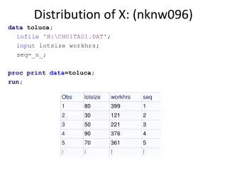
Distribution of X: (nknw096) datatoluca; infile'H:\CH01TA01.DAT'; inputlotsizeworkhrs; seq=_n_; procprintdata=toluca; run;
Distribution of X: Descriptive procunivariatedata=tolucaplot; varlotsizeworkhrs; run;
Distribution of X: Descriptive (4) Stem Leaf # Boxplot 12 0 1 | 11 00 2 | 10 00 2 | 9 0000 4 +-----+ 8 000 3 | | 7 000 3 *--+--* 6 0 1 | | 5 000 3 +-----+ 4 00 2 | 3 000 3 | 2 0 1 | ----+----+----+----+ Multiply Stem.Leaf by 10**+1
Distribution of X: Sequence plot title1h=3'Sequence plot for X with smooth curve'; symbol1v=circle i=sm70; axis1label=(h=2); axis2label=(h=2angle=90); procgplotdata=toluca; plotlotsize*seq/haxis=axis1 vaxis=axis2; run;
Distribution of X: QQPlot title1'QQPlot (normal probability plot)'; procunivariatedata=tolucanoprint; qqplotlotsizeworkhrs / normal (L=1mu=estsigma=est); run;
Quadratic: (nknw100quad.sas) title1h=3'Quadratic relationship'; data quad; do x=1to30; y=x*x-10*x+30+25*normal(0); output; end; procregdata=quad; model y=x; outputout=diagquadr=resid; run;
Quadratic: Example (cont) symbol1v=circle i=rl; axis1label=(h=2); axis2label=(h=2angle=90); procgplotdata=quad; plot y*x/haxis=axis1 vaxis=axis2; run;
Quadratic: Example (cont) symbol1v=circle i=sm60; procgplotdata=quad; plot y*x/haxis=axis1 vaxis=axis2; run;
Heteroscediastic: (nknw100het.sas) title1h=3'Heteroscedastic'; axis1label=(h=2); axis2label=(h=2angle=90); Datahet; do x=1to100; y=100*x+30+10*x*normal(0); output; end; procregdata=het; model y=x; run;
Heteroscediastic: Example (cont) symbol1v=circle i=sm60; procgplotdata=het; plot y*x/haxis=axis1 vaxis=axis2; run;
Outlier: Example1 (nknw100out.sas) title1h=3'Outlier at x=50'; axis1label=(h=2); axis2label=(h=2angle=90); dataoutlier50; do x=1to100by5; y=30+50*x+200*normal(0); output; end; x=50; y=30+50*50 +10000; d='out'; output; procprintdata=outlier50; run;
Outlier: Example1 (cont) Code: Without outlier: With outlier: procregdata=outlier50;procregdata=outlier50; model y=x;model y=x; where d ne 'out';
Outlier: Example1 (cont) symbol1v=circle i=rl; procgplotdata=outlier50; plot y*x/haxis=axis1 vaxis=axis2; run;
Outlier: Example2 (nknw100out.sas) title1h=3'Outlier at x=100'; dataoutlier100; do x=1to100by5; y=30+50*x+200*normal(0); output; end; x=100; y=30+50*100 -10000; d='out'; output; procprintdata=outlier100; run;
Outlier: Example2 (cont) Code: Without outlier: With outlier: procregdata=outlier100;procregdata=outlier100; model y=x;model y=x; where d ne 'out';
Outlier: Example2 (cont) symbol1v=circle i=rl; procgplotdata=outlier100; plot y*x/haxis=axis1 vaxis=axis2; run;
Toluca: Residual Plot (nknw106a.sas) title1h=3'Toluca Diagnostics'; datatoluca; infile'H:\My Documents\Stat 512\CH01TA01.DAT'; inputlotsizeworkhrs; procregdata=toluca; modelworkhrs=lotsize; outputout=diagr=resid; run; symbol1v=circle cv = red; axis1label=(h=2); axis2label=(h=2angle=90); procgplotdata=diag; plotresid*lotsize/ vref=0haxis=axis1 vaxis=axis2; run; quit;
Normality: Toluca (nknw106b.sas) title1h=3'Toluca Diagnostics'; datatoluca; infile'H:\My Documents\Stat 512\CH01TA01.DAT'; inputlotsizeworkhrs; procprintdata=toluca; run; procregdata=toluca; modelworkhrs=lotsize; outputout=diagr=resid; run; procunivariatedata=diagplotnormal; varresid; histogramresid / normalkernel; qqplotresid / normal (mu=est sigma=est); run;
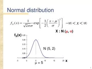
Normal: (nknw100norm.sas) %let mu = 0; %let sigma=10; title1'Normal Distribution mu='&mu' sigma='σ data norm; do x=1to100; y=100*x+30+rand('normal',&mu,&sigma); output; end; procregdata=norm; model y=x; outputout=diagnormr=resid; run; symbol1v=circle i=none; procunivariatedata=diagnorm plotnormal; varresid; histogramresid / normalkernel; qqplotresid / normal (mu=est sigma=est); run;
Normal: (cont) Normal Distribution mu=0 sigma=10
Normality: failure (nknw100nnorm.sas) title1'Right Skewed distribution'; data expo; do x=1to100; y=100*x+30+exp(2)*rand('exponential'); output; end; procregdata=expo; model y=x; outputout=diagexpor=resid; run; symbol1v=circle i=none; procunivariatedata=diagexpoplotnormal; varresid; histogramresid / normalkernel; qqplotresid / normal (mu=est sigma=est); run;
Normality: nongraphical procunivariatedata=diagy normal; varresid; run; Toluca:
Transformations (Y) Y’ = Y’ = log10 Y Y’ = 1/Y Note: a simultaneous transformation on X may also be helpful or necessary.
Box-Cox: Plasma (boxcox.sas) Y = Plasma level of polyamine X = Age of healthy children n = 25
Box-Cox: Example (Input) dataorig; input age plasma @@; cards; 0 13.44 0 12.84 0 11.91 0 20.09 0 15.60 1 10.11 1 11.38 1 10.28 1 8.96 1 8.59 2 9.83 2 9.00 2 8.65 2 7.85 2 8.88 3 7.94 3 6.01 3 5.14 3 6.90 3 6.77 4 4.86 4 5.10 4 5.67 4 5.75 4 6.23 ; procprintdata=orig; run;
Box-Cox: Example (Y vs. X) title1h=3'Original Variables'; axis1label=(h=2); axis2label=(h=3angle=90); symbol1v=circle i=rl; procgplotdata=orig; plot plasma*age/haxis=axis1 vaxis=axis2; run;
Box-Cox: Example (regression) procregdata=orig; model plasma=age; outputout = notransr = resid; run;
Box-Cox: Example (resid vs. X) symbol1i=sm70; procgplotdata = notrans; plotresid*age / vref = 0haxis=axis1 vaxis=axis2;
Box-Cox: Example (QQPlot) procunivariatedata=notransnoprint; varresid; histogramresid/normalkernel; qqplotresid/normal (mu = est sigma=est); run;
Box-Cox: Example (find transformation) proctransregdata = orig; modelboxcox(plasma)=identity(age); run;
Box-Cox: Example (calc transformation) title1'Transformed Variables'; data trans; setorig; logplasma = log(plasma); rsplasma = plasma**(-0.5); procprintdata = trans; run;
Box-Cox: Log (Y vs. X) symbol1i=rl; procgplotdata = logtrans; plotlogplasma * age/haxis=axis1 vaxis=axis2; run;
Box-Cox: Log (regression) procregdata = trans; modellogplasma = age; outputout = logtransr = logresid; run;