NetCDF and Self-Describing Data
NetCDF and Self-Describing Data. Kate Hedstrom January 2010 http://www.arsc.edu/~kate/NetCDF/. Older File Formats. ASCII Easy to read if small Can get large Have to know structure to make plots Slow to read, write Binary Smaller, faster than ASCII Have to know structure

NetCDF and Self-Describing Data
E N D
Presentation Transcript
NetCDF and Self-Describing Data Kate Hedstrom January 2010 http://www.arsc.edu/~kate/NetCDF/
Older File Formats • ASCII • Easy to read if small • Can get large • Have to know structure to make plots • Slow to read, write • Binary • Smaller, faster than ASCII • Have to know structure • Not necessarily portable • Opaque from outside application • Example: 9-track tape with ocean data
Metadata • Problems parsing older files has lead to the development of metadata: • Data about the data • File contains data but also • Name of fields • Dimensions • Type • Units • Special values • Global attributes, such as title, source, history, version, etc.
XML • An ASCII format which can contain all the metadata you want in the form of a DTD or Schema • Very cool things can be done, translating them with XSLT into other formats • Way too bulky for our geophysical model output needs
Our File Necessities • Binary for speed • Portable • Metadata • Flexible enough for all our data • Open Source • Can be used from all common computer languages
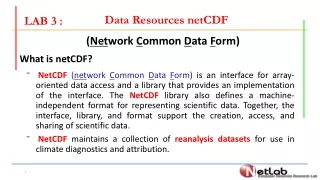
NetCDF and HDF • Network Common Data Format (NetCDF) • http://www.unidata.ucar.edu/packages/netcdf/index.html • Simpler interface • Multi-dimensional arrays, de facto standard for model output for oceans/atmosphere • Hierarchical Data Format (HDF) • http://hdf.ncsa.uiuc.edu/ • Parallel I/O, large files • Collection of file formats • Scientific Data is like NetCDF • Used for NASA images
NetCDF-3 Library • Access to all necessary functionality: • Open old and new files, close files • Create dimensions, variables, attributes • Read and write fields • Inquire about what is in a file • Written in C for portability, speed • Other languages use C interface
Languages • I have used all of these interfaces: • Others: java, ruby, python, GMT, etc.
Programs - ncdump • ASCII dump of all or some of file • Can ask for just header (-h) • Dimensions • Variables and their attributes • Global attributes • Can ask for just one variable (-v time) • Gives the header as well • Surprisingly useful
ncgen • Inverse of ncdump - creates NetCDF file from the ASCII dump • Can be used to modify small files: • ncdump foo.nc > foo.asc • Edit foo.asc • ncgen -o bar.nc foo.asc • Can be used to generate the C / Fortran source for creating the file
ncdump netcdf circle8 { dimensions: len_string = 33 ; len_line = 81 ; four = 4 ; time_step = UNLIMITED ; // (0 currently) num_dim = 3 ; num_nodes = 12 ; num_elem = 13 ; num_el_blk = 1 ; num_el_in_blk1 = 13 ; num_nod_per_el1 = 3 ; num_qa_rec = 1 ;
variables: double time_whole(time_step) ; int connect1(num_el_in_blk1, num_nod_per_el1) ; connect1:elem_type = “TRI3”; double coord(num_dim, num_nodes) ; char coor_names(num_dim, len_string) ; int elem_map(num_elem) ; int elem_num_map(num_elem) ; int node_num_map(num_nodes) ; // global attributes: :api_version = 3.07f ; :version = 2.05f ; :floating_point_word_size = 8 ; :title = “cubit(circle8.nc): 06/05/2003: 14:10:20” ;
data: connect1 = 2, 1, 10, 1, 9, 10, 9, 8, 10, 8, 7, 11, 7, 6, 11, 6, 5, 11, 5, 4, 12, 4, 3, 12, 3, 2, 10, 10, 8, 11, 11, 5, 12, 12, 3, 10, 12, 10, 11 ;
coord = -600, -459.6, -104,2, 300, 563.8, 563.8, 300, -104.2, -459.6, -193.1, 208.0, 154.2, 7.3e-14, 385.7, 590.9, 519.6, 205.2, -205.2, -519.6, -590.9, -385.7, 19.9, -129.8, 238.962035390774, 0, 0, 0, 0, 0, 0, 0, 0, 0, 0, 0, 0 ; coor_names = “x”, “y”, “z” ; elem_map = 1, 2, 3, 4, 5, 6, 7, 8, 9, 10, 11, 12, 13; }
Notes on dump • File contains variable names • File contains dimensions of all variables • Can skip reading unused variables • Global attributes tell how and when file was created • There is an unlimited dimension • Grows as needed • Often used for time records • Only one per file (until version 4)
Reading from Fortran • Declare NetCDF variables, functions include ‘netcdf.inc’ integer ierr, ncid, varid real*8 coord(12,3) • Open the file ierr = nf_open(“circle8.nc”, NF_READ, ncid) • Find out the variable id ierr = nf_inq_varid(ncid, ”coord”, varid) • Read the variable ierr = nf_get_var_double(ncid, varid, coord)
Reading from Fortran • Need to declare coord variable with the right dimensions - can overwrite memory if declared too small • Type of Fortran variable must agree with type in nf_get_var_xxx • If type in file is different from above type, library will do conversion • Arrays in ncdump are C-like: double coord(3,12) • Arrays in Fortran are reversed: real*8 coord(12,3)
Fortran 90 • use netcdf instead of include ‘netcdf.inc’ • Knows type: ierr = nf90_get_var(…) • Need to tell the compiler how to find the module file (in include directory)
NCAR Command Language (NCL) • Scripting language with plotting: http://www.ncl.ucar.edu/ • Open file and read a variable: ncid = addfile(“circle8.nc”, “r”) coord = ncid->coord • Read with type, dimensions, all attributes intact: num_node = dimsizes(coord(0,:)) units = coord@units • C-like array indexing
Cartesian Grid Example • Use NCL to create NetCDF file and display its contents • Design of NetCDF files • This is the hard part • Dimensions • Coordinate variables • Guidelines for attributes
write1.ncl: begin ncid = addfile(“rossby1.nc”, “cw”) x = fspan(-12.0, 12.0, 49) y = fspan(-8.0, 8.0, 33) numx = dimsizes(x) numy = dimsizes(y) ; C order of array dimensions ubar = new((/numy, numx/), “double”) vbar = new((/numy, numx/), “double”) zeta = new((/numy, numx/), “double”) ubar = … ncid->ubar = ubar ncid->vbar = vbar ncid->zeta = zeta end
netcdf rossby1 { dimensions: ncl0 = 33 ; ncl1 = 49 ; ncl2 = 33 ; ncl3 = 49 ; ncl4 = 33 ; ncl5 = 49 ; variables: double ubar(ncl0, ncl1) ; ubar:_FillValue = -9999. ; double vbar(ncl2, ncl3) ; vbar:_FillValue = -9999. ; double zeta(ncl4, ncl5) ; zeta:_FillValue = -9999. ; }
draw1.ncl: load “$NCARG_ROOT/lib/ncarg/nclex/gsun/gsn_code.ncl begin ncid = addfile(“rossby1.nc”, “r”) ubar = ncid->ubar wks = gsn_open_wks(“x11”, “draw”) ; set colorfill resource - otherwise get line contours res = True res@cnFillOn = True cmap = … gsn_define_colormap(wks, cmap) contour = gsn_contour(wks, ubar, res) end
What went right? • Easily created valid NetCDF file • Dimensions are right, _FillValue set automatically • Can easily read a field from the file and plot it up • Half the plotting code is for color contours - black and white line contours are even easier
What could be better? • Created six dimensions when two are needed • Dimension names are not meaningful • _FillValue is the only attribute set • No global attributes • Plot aspect ratio is wrong - no geometry information in file
write2.ncl (part): ; dimensions and attributes ubar!0 = “y” ubar!1 = “x” x!0 = “x” y!0 = “y” x@units = “meter” y@units = “meter” ubar@units = “m/s” zeta@long_name = “Surface Elevation” … ncid->x = x ncid->y = y ncid->ubar = ubar …
netcdf rossby2 { dimensions: x = 49 ; y = 33 ; variables: float x(x) ; x:units = “meter” ; float y(y) ; y:units = “meter” ; double ubar(y, x) ; ubar:units = “m/s” ; ubar:long_name = “Depth-integrated u-velocity” ; ubar:_FillValue = -9999. ; double vbar(y, x) ; : double zeta(y, x) ; zeta:units = “meter” ‘ : }
Changes… Better • The two dimensions are there - with useful names • The two coordinate variables are there • Plot automatically has title (long_name) • Still needs fixing: • Global attributes • Unlimited dimension for multiple time slices
write3.ncl (parts): ; global attributes fileAtt = True fileAtt@title = “Class sample” fileAtt@creation_date = \ systemfunc(“date”) fileAtt@history = “learning NCL” fileattdef(ncid, fileAtt)
write3.ncl (parts): ; unlimited dimension filedimdef(ncid, “time”, -1, True) filevardef(ncid, “time”, “double”, “time”) time = 0.0 time@units = “sec” filevarattdef(ncid, “time”, time) ; (/ /) strips attributes from time ncid->time(0) = (/ time /) : dims = (/”time”, “y”, “x” /) filevardef(ncid, “ubar”, typeof(ubar), dims) filevarattdef(ncid, “ubar”, ubar) ncid->ubar(0,:,:) = (/ubar /)
netcdf rossby3 { dimensions: time = UNLIMITED ; // (1 currently) x = 49 ; y = 33 ; variables: double time(time) ; time:units = “sec” ; float x(x) ; x:units = “meter” ; float y(y) ; y:units = “meter” ; double ubar(time, y, x) ; : // global attributes: :history = “learning NCL” ; :creation_date = “Thu Jul 17 15:08:39 AKDT 2003” ; :title = “Class sample” ; }
Summary of Cartesian Example • We now have our global attributes and an unlimited dimension • All this functionality should be available from any language with a NetCDF interface • We managed to get the plot looking better by setting plot resources, beyond the subject of this talk
Notes on Attributes • Can be set both for the file and for each variable • Not mandatory, but polite • There are “standard” ones such as units, long_name, title, etc. • There are some general and domain-specific guidelines (see NetCDF manual, web page) • Can make up and use own: type=“grid_file” or colorbar=“blues”
Matlab Interface • Available from http://mexcdf.sourceforge.net • Three parts: • mexnc • snctools • NetCDF Toolbox • mexnc is based on the C language interface • Other two use mexnc
More Matlab • Try “help snctools” from the Matlab prompt • Most commonly used are: • nc_varget • nc_varput • nc_attget • nc_attput • nc_dump
NetCDF Operators (NCO) • http://nco.sourceforge.net/ • Concatenate files • Difference files • Average files, records • Extract fields or field subsets • Copy to new file • Copy to another old file • Write to ASCII • Edit attributes, rename variables
Evolution • New HDF5 is incompatible with older HDF4 • Data structures to accommodate satellite data, georeferencing, etc. • Next generation NetCDF-4 is based on HDF5 • More flexible storage • Clearer access routines than HDF5
NetCDF 4 • NetCDF 4.0 contains a new library that calls either NetCDF 3 (compatibility mode) or HDF5 • New functions to get at new functionality, otherwise looks the same as version 3 • Files created will be old style or new HDF5 files - all tools need updating • Still more changes coming in 4.1, 4.2
New Features • Parallel I/O through MPI I/O • More efficient I/O through chunking, compression • Multiple unlimited dimensions • Compound types • Will handle files > 2GB by default, not as special option • New data types • Decide at file creation time if it’s in the new format or not
Conclusions • Converting to NetCDF has been well worth the trouble • Portability • Use of ncdump, nco, etc. • New interfaces from scripting languages can make it simple to use • Converting a new model is easy now that we’ve seen how to do it once - get the fields right first, then fix the attributes • Visualization people will love you!